8 Practical tips for organizing Predictive Soil Mapping
Edited by: T. Hengl, R. A. MacMillan and I. Wheeler
8.1 Critical aspects of Predictive Soil Mapping
Previous chapters in this book have reviewed many of the technical aspects of PSM. For a statistician, following the right procedures and applying the right statistical frameworks will are the key elements of success for a PSM project. In practice, it is really a combination of all elements and aspects that determines a success of a PSM project. In this chapter we provide some practical tips on how to organize work and what to be especially careful about. We refer to these as the critical aspects of PSM projects.
At the end of the chapter we also try to present additional practical tips in the form of check-lists and simple economic analysis, to help readers avoid making unrealistic plans or producing maps that may not find effective use.
8.1.1 PSM main steps
Based on previously presented theory, we can summarize the usual PSM processes as:
Preparation of point data (training data).
Preparation of covariate data (the explanatory variables).
Model fitting and validation (building rules by overlay, model fitting and cross-validation).
Prediction and generation of (currently best-possible) final maps (applying the rules).
Archiving and distribution of maps (usually via soil geographical databases and/or web services).
Updates and improvements (support).
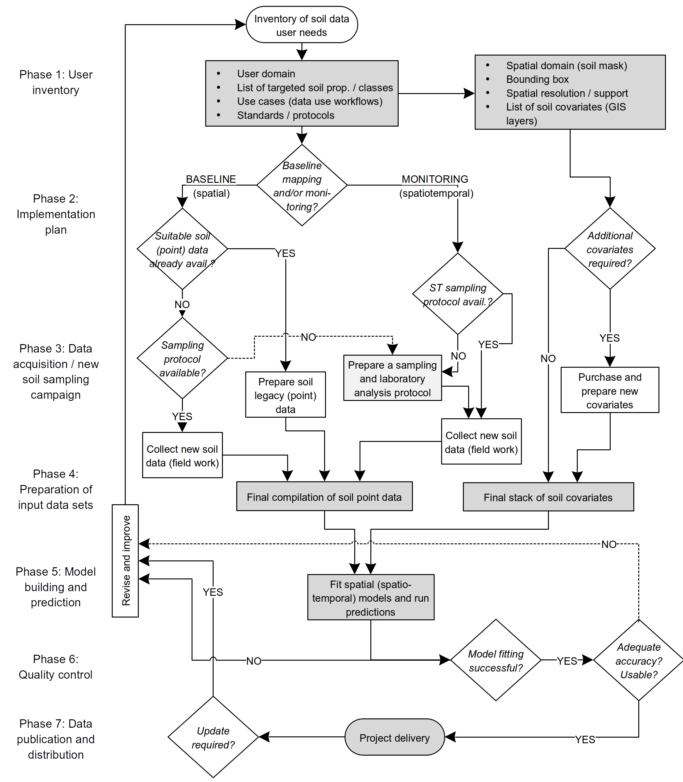
Figure 8.1: General decision tree in a Predictive Soil Mapping project.
An even more comprehensive list of steps in PSM projects is given in Fig. 8.1, which also includes market/user-domain researcher and might be also used for soil monitoring projects.
In principle, we recognize three main types of PSM projects:
PSM projects in new, previously unmapped, areas — no point observations or samples currently exist.
PSM projects using legacy points — sufficient point data to support PSM exist and are available, but no previous PSM modelling has been implemented for this area.
PSM projects aimed at optimizing predictions and usability — Previous PSM models have already been completed but previous results can still be improved / optimized.
If point data are not available, then collecting new point data, via field work and laboratory analysis will usually consume a majority of any PSM project budget (PSM projects type A). Otherwise, if point data are already available (and only need to be imported and harmonized), the most time consuming part of PSM will likely be preparation of covariate data layers (PSM projects type B). Predictions can also take a long time and computing costs per update can be significant (see further sections). Personnel costs can be more significant than server costs as programming can require weeks of staff time. However, if programming is done at a high level (e.g. through generic functions and objects), subsequent updates should require less personnel time as predictions can be increasingly automated.
Another aspect of PSM is the time dimension i.e. will maps be continuously updated or do they need to produced only once and then remain relevant and useful for years (often up to decades), so that PSM projects can also be classified into:
PSM projects for the purpose of mapping static (stable) spatial patterns only.
PSM projects for the purpose of one-time change detection (e.g. two time intervals).
PSM projects for the purpose of monitoring soil conditions / status (continuous updates at regular intervals).
To date, almost all conventional soil mapping ignores time and change and instead tries to assume that soil properties are static and persist through time virtually unaltered. Increasingly, however, new generation PSM projects aim to monitor changes in soil resources, with special focus given to changes in soil organic carbon, soil nutrients, soil moisture and similar (Fig. 8.2). For PSM project type III spatio-temporal prediction models can be used (as in meteorology for example), but then this requires that sufficient training data are available in both the space and time domains e.g. at least five measurement intervals / repetitions.

Figure 8.2: Types of PSM projects depending on whether maps are generated for single usage, or for detecting change or soil monitoring.
8.1.2 PSM input and output spatial data layers
In PSM, there are, in principle, three (3) main types of spatial input layers (Hengl, Mendes de Jesus, et al. 2017):
Soil samples (usually points or transects) are spatially incomplete. They are used as evidence in generating spatial predictions. In vertical and horizontal dimensions, soil points might refer to volumes i.e. have a block support. Often only the horizontal (2D) support is mentioned, and the 3D support has to be inferred from the description of the depth slice(s) sampled.
Soil mask i.e.a raster map delineating the spatial domain of interest for PSM. Commonly derived from a land cover map with water bodies, permanent ice and similar removed from predictions.
Covariates i.e. grid maps that depict environmental conditions. Ideally all covariates are “stacked” to exactly match the same grid and all missing values and inconsistencies are resolved prior to PSM.
And three (3) main types of spatial output layers:
Spatial predictions of (primary) soil variables that are spatially complete i.e. are produced and available for the entire extent of the soil mask.
Maps of (secondary) soil variables which are derived using calculations applied to combinations of the primary predicted soil variables. These are usually less expensive to produce, by an order of magnitude, than spatial predictions of primary soil variables.
Maps quantifying uncertainty in terms of prediction error, prediction interval, confusion index or similar metrics. These may be derived at the same time as predictions are made or can be made completely independently of predictions.
Each element of the map types listed above needs to have a consistent spatio-temporal reference, which typically includes:
Geographic location in local or geographic coordinates (for global modelling we usually prefer initial georeferencing that uses longitude and latitude in the WGS84 coordinate system);
Depth interval expressed in cm from the land surface (upper and lower depth) for layers and point depth for point predictions;
Support size or referent soil volume (or voxel) i.e. the horizontal sampling area multiplied by the thickness of the sampling block e.g. 30 \(\times\) 30 \(\times\) 0.3 m.
Temporal reference i.e. a begin and an end date/time of the period of measurements/estimations. Specifying exact spatial and temporal references in the metadata can is vital for optimal production and use of maps.
Spatial predictions of primary soil properties can be used to:
Derive spatial aggregates (upscaling to coarser resolution).
Derive vertical aggregates e.g. mean pH in 0–100 cm of soil (for this we usually recommend using the trapezoidal rule as explained in Hengl, Mendes de Jesus, et al. (2017)).
Derive secondary soil properties e.g. available water capacity, organic carbon stock etc.
Spatial predictions of primary soil variables and derived soil variables are meant to be used for decision making and further modeling i.e. they are used to construct a Soil Information System once all values of all variables are known for all pixels within the soil mask. A SIS should ideally provide information that can directly support input to modeling, planning and decision-making.
8.2 Technical specifications affecting the majority of production costs
The majority of the costs of a PSM project are controlled by the following:
Spatial resolution (commonly 30 m, 100 m or 250 m): Spatial resolution is crucial in determining the total costs of PSM, especially in terms of computing, storage, network traffic and hardware requirements. Changing the spatial resolution from 100 to 30 m means that about 10 times more pixels will need to be produced, stored and shared via the network. This does not always imply that the costs of PSM will also be 10 times greater than for a 100 m resolution project, but the increase in costs is often going to follow a quadratic function. Also note that, for even finer resolutions e.g. 5 m, very limited free public covariate data are available and additional purchases of commercial RS products will typically be required. For example the latest 12 m resolution WorldDEM (https://worlddem-database.terrasar.com/) can cost up to 10 USD per square km, which can increase PSM costs significantly.
List of target variables and their complexity: Some PSM projects focus on mapping 1–2 soil variables only, and as such can be rather straightforward to implement. Any PSM project that requires creation of a complete Soil Information System (tens of quantitative soil variables and soil types), will definitely demand more effort and hence potentially significantly increase costs. Typically, evaluation and quality control of maps in a SIS requires an analyst to open and visually compare patterns from different maps and to make use of considerable empirical knowledge of soils. Costs of production can also be significantly increased depending on whether lower and upper prediction intervals are required. As with increasing spatial resolution, requesting lower and upper prediction intervals means that two times more pixels will need to be produced.
Targeted accuracy/quality levels: Often the agencies that order spatial soil information expect that predictions will achieve some desired accuracy targets. Accuracy of predictions can, indeed, often be improved (but only up to a certain level), by simply improving the modelling framework (PSM projects type C). In practice, if a contractor requires significant improvements in accuracy, then this often means that both additional point records and improved covariate data (for example at finer spatial resolution) will need to be collected and/or purchased. This can often mean that the original budget will have to be increased until the required accuracy level can be reached.
List of targeted services / user domain: Is the goal of the PSM project to produce data only, or to serve this data for a number of applications (use-cases)? How broad is the user domain? Is the data being made for a few targeted clients or for the widest possible user base? Is high traffic expected and, if so, how will the costs of hosting and serving the data and processes be met? Producing a robust, scalable web-system that can serve thousands of users at the same time requires considerable investments in programming and maintenance.
Commercialization options: Commercialization of data and services can also significantly increase costs, since the development team needs to prepare also workflows where invoices and bills are generated on demand, or where efficient support and security are now critically important. Even though many companies exist that offer outsourcing of this functionality, many organizations and companies prefer to have full control of the commercialization steps, hence such functionality needs to be then developed internally within the project or organization.
8.2.1 Field observations and measurements
Observations and measurements (O&M) are at the heart of all advances in scientific endeavor. One cannot describe, or attempt to understand, what one cannot see, or measure. Great leaps in scientific understanding have always followed from major improvements in the ability to see, and measure, phenomenon or objects. Think of the telescope and astronomy, the microscope and microbiology, the X-ray and atomic structure or crystallography and so on.
In the area of resource inventories, observations and measurements carried out in the field (field data) provide the evidence critical to developing the understanding of spatial patterns and spatial processes that underpins all models that predict the spatial distribution of properties or classes. This applies equally to subjective, empirical mental, or conceptual, models and objective, quantitative statistical models. The more and better the observations and measurements we obtain, the better will be our ability to understand and predict spatial patterns of soils and other natural phenomena. Consider here some general observations on how to maximize efficiency of O&M:
For maximum utility, field data should be objective and reproducible.
They should be collected using some kind of unbiased sampling design that supports reproducibility and return sampling (Brus 2019; Malone, Minansy, and Brungard 2019).
They should be located as accurately as possible in both space (geolocation) and time (temporal location).
They should describe and measure actual conditions in their present state (and current land use) and not in some assumed natural, climax or equilibrium condition.
They should capture and permit description of spatial and temporal variation across multiple spatial scales and time frames.
It is widely assumed that collecting new field data to produce new and improved inventory products is prohibitively expensive and will never be possible or affordable in the foreseeable future. Consequently, most current projects or programs that aim to produce new maps of soils or other terrestrial entities have explicitly embraced the assumption that the only feasible way to produce new soil maps is to locate, and make use of, existing legacy data consisting of previously reported field observations or existing laboratory analysed field samples. However, recent activities in Africa (www.Africasoils.net), for example, have demonstrated conclusively that it is feasible, affordable and beneficial to collect new field observations and samples and to analyse new soil samples affordably and to a high standard (Shepherd and Walsh 2007).
8.2.2 Preparation of point data
Import of basic O&M field data (e.g. soil point data) can be time consuming and require intensive, often manual, checking and harmonization. Communicating with the original data producers is highly recommended to reduce errors during import. Getting original data producers involved can be best achieved by inviting them to become full participants ( e.g. join in joint publications) or by at least providing adequate and visible acknowledgement (e.g. listing names and affiliations in metadata or on project websites).
Documenting all import, filtering and translation steps applied to source data is highly recommended, as these steps can then be communicated to the original field data producers to help filter out further bugs. We typically generate a single tabular object with the following properties as our final output of point data preparation :
Consistent column names are used; metadata explaining column names is provided,
All columns contain standardized data (same variable type, same measurement units) with harmonized values (no significant bias in values from sub-methods),
All artifacts, outliers and typos have been identified and corrected to the best of our ability,
Missing values have been imputed (replaced with estimated values) as much as possible,
Spatial coordinates, including depths, (x,y,z) are available for all rows (point locations).
8.2.3 Preparation of covariates
As mentioned previously, preparation of covariate layers can require significant effort, even if RS data is publicly available and well documented. For example, MODIS land products are among the most used RS layers for global to regional PSM. Using raw reflectance data, such as the mid-infrared MODIS bands from a single day can, however, be of limited use for soil mapping in areas with dynamic vegetation, i.e. with strong seasonal changes in vegetation cover. To account for seasonal fluctuation and for inter-annual variations in surface reflectance, we instead advise using long-term temporal signatures of the soil surface derived as monthly averages from long-term MODIS imagery (18+ years of data). We assume here that, for each location in the world, long-term average seasonal signatures of surface reflectance or vegetation index provide a better indication of site environmental characteristics than just a single day snapshot of surface reflectance. Computing temporal signatures of the land surface requires a large investment of time (comparable to the generation of climatic images vs temporary weather maps), but it is possibly the only way to effectively represent the cumulative influence of living organisms on soil formation (Hengl, Mendes de Jesus, et al. 2017).
Typical operations to prepare soil covariates for PSM thus include:
Downloading the original source RS data,
Filtering missing pixels using neighborhood filters and/or simple rules,
Running aggregation functions (usually via some tiling system),
Running hydrological and morphological analysis on source DEM data
Calculation of a Gaussian pyramid, for some relevant covariates, at multiple coarser resolutions, in order to capture multi-scale variation at appropriate (longer range) process scales.
Preparing final mosaics to be used for PSM (e.g. convert to GeoTIFFs and compress using internal compression
"COMPRESS=DEFLATE"or similar),
For processing the covariates we currently use a combination of Open Source GIS software, primarily SAGA GIS, GRASS GIS, Whitebox tools, R packages raster, sp, GSIF and GDAL for reprojecting, mosaicking and merging tiles. SAGA GIS and GDAL were found to be highly suitable for processing massive data sets, as parallelization of computing was relatively easy to implement.
Preparation of covariate layers is completed once:
all layers have been resampled to exactly the same grid resolution and spatial reference frame (downscaling or aggregation applied where necessary),
all layers are complete (present for >95% of the soil mask at least; the remaining 5% of missing pixels can usually be filled-in using some algorithm),
there are no visibly obvious artifacts or blunders in the input covariate layers,
8.2.4 Soil mask and the grid system
We recommend using a raster mask file to define the spatial domain of interest (i.e. total number of pixels to be mapped), and the spatial reference framework for PSM. The mask file defines the maximum extent, or bounds, of the area for which predictions will be made. It also identifies any grid cells, within the maximum bounds, which are to be excluded from prediction for various reasons (e.g. water, ice or human disturbance). Finally, the mask file establishes the resolution (pixel size) and spatial coordinate system that all other layers included in the analysis must conform to, to ensure consistent overlay of all grids. In most of our PSM projects we typically restrict ourselves to making predictions only for pixels that exhibit some evidence of having photosynthetically active vegetative cover at some point in time. We tend to exclude from prediction any grid cells that have no evidence of vegetative cover at any time, such as permanent bodies of water or ice, bare rock and man made features such as roads, bridges and buildings. A generic definition of a soil mask can differ somewhat from the one we use, but this has been our practice.
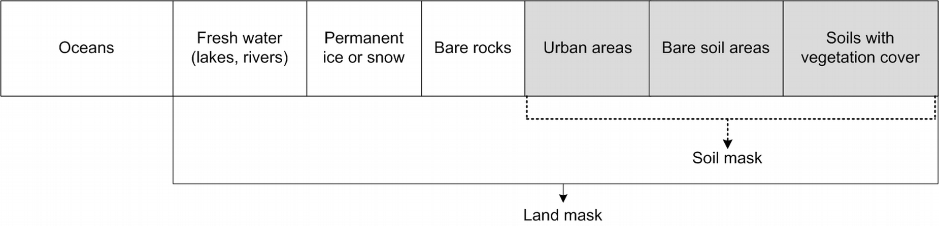
Figure 8.3: Example of a soil (land) mask scheme.
From the perspective of global soil mapping, any terrestrial location on Earth can be considered to belong to one and only one of six categories (excluding oceans):
A. Fresh water (lakes, rivers)
B. Permanent ice or snow
C. Bare rocks
D. Urban areas
E. Bare soil areas
F. Soils with vegetation cover
This gives the following formulas:
F = Land mask - ( A + B + C + D + E )
Soil mask = D + E + F
Hence the values in the soil mask can be typically coded as:
0 = NA or non-soil
1 = soils with vegetation cover
2 = urban areas
3 = bare soil areas
If no other layers are available, global maps of land cover can be used to produce a soil mask file (following the simple formula from above). Some known global land cover layers are:
300 m resolution: ESA CCI Land cover — 300 m annual global land cover time series from 1992 to 2015 (https://www.esa-landcover-cci.org/),
100 m resolution: ESA PROBA-V 100 m land cover map (http://land.copernicus.eu/global),
30 m resolution: Chinese GLC data product (GlobeLand30) with 10 classes for the years 2000 and 2010 (http://www.globallandcover.com),
Using widely accepted, published, global land cover maps to define a soil mask is highly recommended. This allows users to validate the maps and also ensures future consistency in case there is a need in the future to merge multiple maps covering larger areas.
Another important technical consideration for a PSM project is the grid system. The grid system is defined by the bounding box, pixel size and number of rows and columns:
- Xmin, Xmax, Ymin, Ymax,
- Spatial resolution in m (projected),
- Spatial resolution in DD,
- Number of rows (X) and columns (Y),
Maps referenced by geographical coordinates (EPSG:4326; used by the GPS satellite navigation system and for NATO military geodetic surveying) have spatial resolution given in abstract decimal degrees (which do not relate 1:1 with metric resolution). Some standard spatial resolutions (in decimal degrees) can be derived using the following simple rules of thumb (d.d. = decimal degrees):
30 m ≈ 1/4000 d.d. = 0.00025
100 m ≈ 1/1200 d.d. = 0.0008333333
250 m ≈ 1/480 d.d. = 0.002083333
500 m ≈ 1/240 d.d. = 0.004166667
1 km ≈ 1/120 d.d. = 0.008333333
Again, these are only approximate conversions. Differences in resolution in x/y coordinates in projected 2D space and geographical coordinates can be large, especially around poles and near the equator.
Another highly recommended convention is to use some widely accepted Equal area projection system for all intermediate and final output maps. This ensures the best possible precision in determining area measures, which is often important e.g. for derivation of total stocks, volumes of soil and soil components and similar. Every country tends to use a specific equal area projection system for it’s mapping, which is usually available from the National mapping agency. For continental scale maps we recommend using e.g. the Equi7 grid system. Some recognized advantages of the Equi7 Grid system are:
The projections of the Equi7 Grid are equidistant and hence suitable for various geographic analyses, especially for derivation of buffer distances and for hydrological DEM modeling, i.e. to derive all DEM-based soil covariates,
Areal and shape distortions stemming from the Equi7 Grid projection are relatively small, yielding a small grid oversampling factor,
The Equi7 Grid system ensures an efficient raster data storage while suppressing inaccuracies during spatial transformation.
8.2.5 Uncertainty of PSM maps
For soil maps to be considered trustworthy and used appropriately, producers are often required to report mapping accuracy (usually per soil variable) and identify limitations of the produced maps. There are many measures of mapping accuracy, but usually these can be grouped around the following two approaches:
Prediction intervals at each prediction point, i.e. lower and upper limits for 90% probability range.
Global (whole-map) measures of the mapping accuracy (RMSE, ME, CCC, z-scores, variogram of CV residuals).
The mean width of prediction intervals and global measures of mapping accuracy should, in principle, match, although it is possible that the mean width of prediction intervals can often be somewhat wider (a consequence of extrapolation). In some cases, measures of uncertainty can be over-optimistic or biased (which will eventually be exposed by new observations), which can decrease confidence in the product, hence providing realistic estimates of uncertainty of uncertainty is often equally as important as optimizing predictions.
Common approaches to improving the accuracy of predicted maps i.e. narrowing down the prediction intervals are to (a) collect new additional data at point locations where models perform the poorest (e.g. exhibit the widest prediction intervals), and (b) invest in preparing more meaningful covariates, especially finer resolution covariates. Technical specifications, however, influence the production costs and have to be considered carefully as production costs can significantly increase with e.g. finer pixel size. Aiming at 30% lower RMSE might seem trivial but the costs of such improvement could exceed the original budget by several times (Hengl, Nikolić, and MacMillan 2013).
8.2.6 Computing costs
To achieve efficient computing, experienced data scientists understand the importance of utilizing the full capacity of the available hardware to its maximum potential (100%). This usually implies that:
the most up-to-date software is used for all computing tasks,
the software is installed in such a way that it can achieve maximum computing capacity,
any function, or process, that can be parallelized in theory is also parallelized in practice,
running functions on the system will not result in system shutdowns, failures or artifacts,
As mentioned previously, applying PSM for large areas at finer resolutions (billions of pixels) benefits from use of a high performance computing (HPC) server to run overlay, model fitting and predictions and to then generate mosaics. The current code presented in this PSM with R book is more or less 90% optimized so that running of the most important functions can be easily scaled up. The total time required to run one global update on a single dedicated HPC server (e.g. via Amazon AWS) for a soil mask that contains >100 million pixels can require weeks of computing time. Copying and uploading files can also be a lengthy process.
A configuration we adopt, and recommend, for processing large stacks of grids with a large number of evidence points is e.g. the OVH server:
- EG-512-H (512GB RAM takes 3 weeks of computing; costs ca € 950,00 per month)
An alternative to using OVH is the Amazon AWS (Fig. 8.4). Amazon AWS server, with a similar configuration, might appear to cost much more than an OVH server (especially if used continuously over a month period), but Amazon permits computing costs to be paid by the hour, which provides more flexibility for less intensive users. As a rule of thumb, a dedicated server at Amazon AWS, if used continuously 100% for the whole month, could cost up to 2.5 times more than an OVH server.
The recommended server for running PSM on Amazon AWS to produce predictions for billions of pixels is:
- AWS m4.16xlarge ($3.84 per Hour);
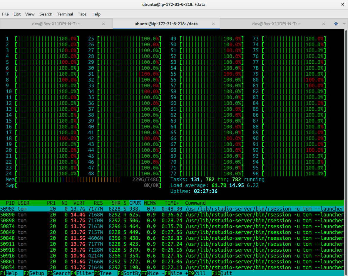
Figure 8.4: Example of an AWS dedicated server running spatial predictions on 96 threads and using almost 500GB of RAM. Renting out this server can cost up to 8 USD per hour.
A HPC server should also have at least 2–3TB of hard disk space to host all input and output data. In addition to computing costs, one also needs to carefully consider web hosting and web traffic costs. For large data sets these can almost equal actual computing production costs.
8.3 Final delivery of maps
8.3.1 Delivery data formats
A highly suitable and flexible data format for delivering raster images of soil variables is GeoTIFF. We prefer using this format for sharing raster data for the following reasons (Mitchell and GDAL Developers 2014):
It is GDAL’s default data format and much functionality for subsetting, reprojecting, reading and writing GeoTIFFs already exists (see GDAL utils).
It supports internal compression via creation options (e.g.
COMPRESS=DEFLATE).Extensive overlay, subset, index, translate functionality is available via GDAL and other open source software. Basically, the GeoTIFF format functions as a raster DB.
By exporting spatial data to GeoTiffs, one can create a soil spatial DB or a soil information system. This does not necessarily mean that its targeted users will be able to find all information without problems and/or questions. The usability and popularity of a data set reflect many considerations in addition to data quality.
Another useful aspect of final delivery of maps is compression of the GeoTIFFs. To avoid large file sizes, we recommend always using integers inside GeoTIFF formats because floating point formats can result in increases in file sizes of up four times (with no increase in accuracy). This might require multiplication of original values of the soil property of interest by 10 or 100, in order to maintain precision and accuracy (e.g. multiply pH values by 10 before exporting your raster into integer GeoTIFF format).
8.3.2 General recommendations
Even maps of perfect quality might still not attract users, if they are not properly designed. Some things to consider to increase both use and usability of map data are:
Make a landing page for your map data that includes: (a) simple access/download instructions, (b) screenshots of your data in action (people prefer visual explanations with examples), (c) links to key documents explaining how the data were produced, and (d) workflows explaining how to request support (who to contact and how).
Make data accessible from multiple independent systems e.g. via WCS, FTP and through a mirror site (in case one of the access sites goes offline). This might be inefficient considering there will be multiple copies of the same data, but it can quadruple data usage.
Explain the data formats used to share data, and provide tutorials, for both beginners and advanced users, that instruct how to access and use the data.
Consider installing and using a version control system (or simply use github or a similar repository) so that the users can track earlier versions of map data.
Consider closely following principles of reproducible research (all processing steps, inputs and outputs are accessible). For example, making the R code available via github so that anyone is theoretically able to reproduce all examples shown in the text. Transparency increases trust.
8.3.3 Technical specifications PSM project
A way to improve planning of a PSM project is to spend more time on preparing the technical aspects of data production. This includes listing the general specifications of the study area, listing target variables and their collection methods, listing covariate layers of interest to be used to improve mapping accuracy and listing targeted spatial prediction algorithms to be compared.
General specifications of the study area include:
- G.1 Project title:
- G.2 PSM project type:
- PSM project in a new area
- PSM project using legacy points
- PSM project aiming at optimizing predictions and usability
- G.3 Target spatial resolution:
- 10 m
- 30 m
- 100 m
- 250 m
- 1000 m
- G.4 Target temporal span (period of interest):
- Begin date,
- End date,
- G.5 Soil mask:
- raster image or land cover classes in the referent land cover map covering the study area
- G.6 Grid definition:
- Xmin,
- Ymin,
- Xmax,
- Ymax,
- G.7 Target projection system:
- proj4 code,
- G.8 Total area:
- in square-km,
- G.9 Inspection density (observations per square-km):
- Detailed soil profiles,
- Soil semi-profiles,
- Top-soil / sub-soil samples (with laboratory analysis),
- Quick observations (no lab data),
- G.10 Total budget (planned):
- G.11 Total pixels in millions:
- amount of pixels for all predictions
- G.12 Total planned production costs per 1M pixels (divide G.10 by G.11):
- G.13 Target data license:
- G.14 Target user groups and workflows (targeted services):
- G.15 Further updates of maps:
- Continuous updates in regular intervals,
- Two prediction time intervals (start, end period),
- No updates required except fixes and corrections,
- G.16 Commercialization of the PSM outputs:
- No commercial data nor services,
- Commercial data products,
- Commercial services,
- G.17 Support options:
- Dedicated staff / live contact,
- Mailing list,
- Github / code repository issues,
8.3.4 Standard soil data production costs
Standard production costs can be roughly split into three main categories:
Fixed costs (e.g. project initiation, equipment, materials, workshops etc),
- Variable data production costs expressed per:
- M (million) of pixels of data produced,
- Number of points samples,
- Number of variables modeled,
Data maintenance and web-serving costs, usually expressed as monthly/yearly costs,
Although in the introduction chapter we mentioned that the production costs are mainly a function of grid resolution i.e. cartographic scale, in practice several other factors determine the total costs. Standard soil data production costs (approximate estimates) per soil data quality category (see below) are connected to the quality level of the output maps. Consider that there are four main quality levels:
L0 = initial product with only few soil properties, no quality/accuracy requirements,
L1 = final complete product with no quality/accuracy requirements,
L2 = final complete product matching standard accuracy requirements,
L3 = final complete certified product according to the ISO or similar standards.
| Project_type | L0 | L1 | L2 | L3 |
|---|---|---|---|---|
| New area (single state) | 500-1000 | 1,000-5,000 | 5,000-50,000 | >50,000 |
| Using legacy points (single state) | 0.8 | 2 | 2–50 | >50 |
| Aiming at optimizing predictions | 0.5 | 0.8 | NA | NA |
| Aiming at change detection (two states) | NA | NA | NA | NA |
| Aiming at monitoring (multiple states) | NA | NA | NA | NA |
To convert average costs / M pixels to total costs we run the following calculus:
Pixel resolution = 100 m
USA48 area = 8,080,464.3 square-km
Total pixels 6 depths 3 soil properties = 14,544 Mpix
Average production costs (L1) = 0.8 US$ / Mpix
Total production costs PSM projects using legacy points (single state, L1) = 11,635 US$
Average production costs (L2) = 2 US$ / Mpix
Total production costs PSM projects using legacy points (single state, L2) = 29,088 US$
Note: this is a very generic estimate of the production costs and actual numbers might be significantly different. Additional fixed costs + monthly/yearly costs need to be added to these numbers to account also for any web hosting, support or update costs.
Compare these costs with the following standard estimated costs to deliver completed conventional manual soil survey products (see also section 5.3.7):
8.4 Summary notes
Predictive soil mapping applies statistical and/or machine learning techniques to fit models for the purpose of producing spatial and/or spatiotemporal predictions of soil variables i.e. to produce maps of soil properties or soil classes at various resolutions. This chapter identifies and discusses some of the key technical specifications users need to consider to prepare for data production and to obtain realistic estimates of workloads and production costs.
The key technical specifications of a PSM project are considered to consist of defining the following: a soil mask, a spatial resolution, a list of target variables and standard depth intervals (for 3D soil variables), prediction intervals (if required), any secondary soil variables (and how they will be derived) and required accuracy levels. Technical specifications determine the production costs and need to be considered carefully as production costs are sensitive to specifications, (e.g. 3 times finer pixel size can increase production costs up to 10 times, or setting targets such as 30% lower RMSE can increase costs as either more points or more covariates, or both, need to be included. General forms at the end of the chapter provide an example of detailed list of technical specifications in relation to target variables and covariate layers typically used in PSM projects to date.
References
Hengl, T., J. Mendes de Jesus, G. B. M. Heuvelink, M. Ruiperez Gonzalez, M. Kilibarda, A. Blagotic, W. Shangguan, et al. 2017. “SoilGrids250m: Global Gridded Soil Information Based on Machine Learning.” PLoS One 12 (2):e0169748.
Brus, D.J. 2019. “Sampling for digital soil mapping: A tutorial supported by R scripts.” Geoderma 338:464–80. https://doi.org/10.1016/j.geoderma.2018.07.036.
Malone, Brendan P., Budiman Minansy, and Colby Brungard. 2019. “Some Methods to Improve the Utility of Conditioned Latin Hypercube Sampling.” PeerJ 7 (February):e6451. https://doi.org/10.7717/peerj.6451.
Shepherd, K.D., and M.G. Walsh. 2007. “Infrared Spectroscopy — Enabling an Evidence Based Diagnostic Survellance Approach to Agricultural and Environmental Management in Developing Countries.” Journal of Near Infrared Spectroscopy 15:1–19.
Hengl, T., M. Nikolić, and R. A. MacMillan. 2013. “Mapping Efficiency and Information Content.” International Journal of Applied Earth Observation and Geoinformation 22:127–38. https://doi.org/10.1016/j.jag.2012.02.005.
Mitchell, T., and GDAL Developers. 2014. Geospatial Power Tools: GDAL Raster & Vector Commands. Locate Press.
Durana, Patricia J. 2008. “Appendix A: Chronology of the U.S. Soil Survey.” In Profiles in the History of the U.S. Soil Survey, 315–20. Iowa State Press. https://doi.org/10.1002/9780470376959.app1.
Carrick, Sam, Éva-Terézia Vesely, and Allan Hewitt. 2010. “Economic Value of Improved Soil Natural Capital Assessment: A Case Study on Nitrogen Leaching.” In 19th World Congress of Soil Science, 1–6. Brisbane, Australia: IUSS.
MacMillan, R.A., D.E. Moon, R.A. Coupé, and N. Phillips. 2010. “Predictive Ecosystem Mapping (Pem) for 8.2 Million Ha of Forestland,British Columbia, Canada.” In Digital Soil Mapping: Bridging Research, Environmental Application, and Operation, edited by J.L. Boettinger et al., 2:335–54. Progress in Soil Science. Springer. https://doi.org/10.1007/978-90-481-8863-5_27.