5 Statistical theory for predictive soil mapping
Edited by: Hengl T., Heuvelink G.B.M and MacMillan R. A.
5.1 Aspects of spatial variability of soil variables
In this chapter we review the statistical theory for soil mapping. We focus on models considered most suitable for practical implementation and use with soil profile data and gridded covariates, and we provide the mathematical-statistical details of the selected models. We start by revisiting some basic statistical aspects of soil mapping, and conclude by illustrating a proposed framework for reproducible, semi-automated mapping of soil variables using simple, real-world examples.
The code and examples are provided only for illustration. More complex predictive modeling is described in chapter 6. To install and optimize all packages used in this chapter please refer to section 2.5.
5.1.1 Modelling soil variability
Soils vary spatially in a way that is often only partially understood. The main (deterministic) causes of soil spatial variation are the well-known causal factors — climate, organisms, relief, parent material and time — but how these factors jointly shape the soil over time is a very complex process that is (still) extremely difficult to model mechanistically. Moreover, mechanistic modelling approaches require large sets of input data that are realistically not available in practice. Some initial steps have been made, notably for mechanistic modelling of vertical soil variation (see e.g. Finke and Hutson (2008), Sommer, Gerke, and Deumlich (2008), Minasny, McBratney, and Salvador-Blanes (2008), and Vanwalleghem et al. (2010)), but existing approaches are still rudimentary and cannot be used for operational soil mapping. Mainstream soil mapping therefore takes an empirical approach in which the relationship between the soil variable of interest and causal factors (or their proxies) is modelled statistically, using various types of regression models. The explanatory variables used in regression are also known as covariates (a list of common covariates used in soil mapping is provided in chapter 4).
Regression models explain only part of the variation (i.e. variance) of the soil variable of interest, because:
The structure of the regression model does not represent the true mechanistic relationship between the soil and its causal factors.
The regression model includes only a few of the many causal factors that formed the soil.
The covariates used in regression are often only incomplete proxies of the true soil forming factors.
The covariates often contain measurement errors and/or are measured at a much coarser scale (i.e. support) than that of the soil that needs to be mapped.
As a result, soil spatial regression models will often display a substantial amount of residual variance, which may well be larger than the amount of variance explained by the regression itself. The residual variation can subsequently be analysed on spatial structure through a variogram analysis. If there is spatial structure, then kriging the residual and incorporating the result of this in mapping can improve the accuracy of soil predictions (Hengl, Heuvelink, and Rossiter 2007).
5.1.2 Universal model of soil variation
From a statistical point of view, it is convenient to distinguish between three major components of soil variation: (1) deterministic component (trend), (2) spatially correlated component and (3) pure noise. This is the basis of the universal model of soil variation (Burrough and McDonnell 1998; Webster and Oliver 2001, 133):
\[\begin{equation} Z({s}) = m({s}) + \varepsilon '({s}) + \varepsilon ''({s}) \tag{5.1} \end{equation}\]where \(s\) is two-dimensional location, \(m({s})\) is the deterministic component, \(\varepsilon '({s})\) is the spatially correlated stochastic component and \(\varepsilon ''({s})\) is the pure noise (micro-scale variation and measurement error). This model was probably first introduced by Matheron (1969), and has been used as a general framework for spatial prediction of quantities in a variety of environmental research disciplines.
The universal model of soil variation assumes that there are three major components of soil variation: (1) the deterministic component (function of covariates), (2) spatially correlated component (treated as stochastic) and (3) pure noise.
The universal model of soil variation model (Eq.(5.1)) can be further generalised to three-dimensional space and the spatio-temporal domain (3D+T) by letting the variables also depend on depth and time:
\[\begin{equation} Z({s}, d, t) = m({s}, d, t) + \varepsilon '({s}, d, t) + \varepsilon ''({s}, d, t) \tag{5.2} \end{equation}\]where \(d\) is depth expressed in meters downward from the land surface and \(t\) is time. The deterministic component \(m\) may be further decomposed into parts that are purely spatial, purely temporal, purely depth-related or mixtures of all three. Space-time statistical soil models are discussed by Grunwald (2005b), but this area of soil mapping is still rather experimental.
In this chapter, we mainly focus on purely 2D models but also present some theory for 3D models, while 2D+T and 3D+T models of soil variation are significantly more complex (Fig. 5.1).
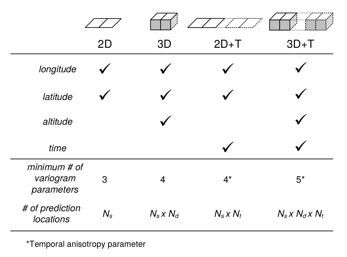
Figure 5.1: Number of variogram parameters assuming an exponential model, minimum number of samples and corresponding increase in number of prediction locations for 2D, 3D, 2D+T and 3D+T models of soil variation. Here “altitude” refers to vertical distance from the land surface, which is in case of soil mapping often expressed as negative vertical distance from the land surface.
One of the reasons why 2D+T and 3D+T models of soil variations are rare is because there are very few point data sets that satisfy the requirements for analysis. One national soil data set that could be analyzed using space-time geostatistics is, for example, the Swiss soil-monitoring network (NABO) data set (Desaules, Ammann, and Schwab 2010), but even this data set does not contain complete profile descriptions following international standards. At regional and global scales it would be even more difficult to find enough data to fit space-time models (and to fit 3D+T variogram models could be even more difficult). For catchments and plots, space-time datasets of soil moisture have been recorded and used in space-time geostatistical modelling (see e.g. Snepvangers, Heuvelink, and Huisman (2003) and Jost, Heuvelink, and Papritz (2005)).
Statistical modelling of the spatial distribution of soils requires field observations because most statistical methods are data-driven. The minimum recommended number of points required to fit 2D geostatistical models, for example, is in the range 50–100 points, but this number increases with any increase in spatial or temporal dimension (Fig. 5.1). The Cookfarm data set for example contains hundreds of thousands of observations, although the study area is relatively small and there are only ca. 50 station locations (Gasch et al. 2015).
The deterministic and stochastic components of soil spatial variation are separately described in more detail in subsequent sections, but before we do this, we first address soil vertical variability and how it can be modelled statistically.
5.1.3 Modelling the variation of soil with depth
Soil properties vary with depth, in some cases much more than in the horizontal direction. There is an increasing awareness that the vertical dimension is important and needs to be incorporated in soil mapping. For example, many spatial prediction models are built using ambiguous vertical reference frames such as predicted soil property for “top-soil” or “A-horizon”. Top-soil can refer to different depths / thicknesses and so can the A-horizon range from a few centimeters to over one meter. Hence before fitting a 2D spatial model to soil profile data, it is a good idea to standardize values to standard depths, otherwise soil observation depth becomes an additional source of uncertainty. For example soil organic carbon content is strongly controlled by soil depth, so combining values from two A horizons one thick and the other thin, would increase the complexity of 2D soil mapping because a fraction of the variance is controlled by the depth, which is ignored.
The concept of perfectly homogeneous soil horizons is often too restrictive and can be better replaced with continuous representations of soil vertical variation i.e. soil-depth functions or curves. Variation of soil properties with depth is typically modelled using one of two approaches (Fig. 5.2):
Continuous vertical variation — This assumes that soil variables change continuously with depth. The soil-depth relationship is modelled using either:
Parametric model — The relationship is modelled using mathematical functions such as logarithmic or exponential decay functions.
Non-parametric model — The soil property changes continuously but without obvious regularity with depth. Changes in values are modelled using locally fitted functions such as piecewise linear functions or splines.
Abrupt or stratified vertical variation — This assumes that soil horizons are distinct and homogeneous bodies of soil material and that soil properties are constant within horizons and change abruptly at boundaries between horizons.
Combinations of the two approaches are also possible, such as the use of exponential decay functions per soil horizon (B. Kempen, Brus, and Stoorvogel 2011).
Parametric continuous models are chosen to reflect pedological knowledge e.g. knowledge of soil forming processes. For example, organic carbon usually originates from plant production i.e. litter or roots. Generally, the upper layers of the soil tend to have greater organic carbon content, which decreases continuously with depth, so that the soil-depth relationship can be modelled with a negative-exponential function:
\[\begin{equation} {\texttt{ORC}} (d) = {\texttt{ORC}} (d_0) \cdot \exp(-\tau \cdot d) \tag{5.3} \end{equation}\]where \(\texttt{ORC}(d)\) is the soil organic carbon content at depth (\(d\)), \({\texttt{ORC}} (d_0)\) is the organic carbon content at the soil surface and \(\tau\) is the rate of decrease with depth. This model has only two parameters that must be chosen such that model averages over sampling horizons match those of the observations as closely as possible. Once the model parameters have been estimated, we can easily predict concentrations for any depth interval.
Consider for example this sample profile from Nigeria:
lon = 3.90; lat = 7.50; id = "ISRIC:NG0017"; FAO1988 = "LXp"
top = c(0, 18, 36, 65, 87, 127)
bottom = c(18, 36, 65, 87, 127, 181)
ORCDRC = c(18.4, 4.4, 3.6, 3.6, 3.2, 1.2)
munsell = c("7.5YR3/2", "7.5YR4/4", "2.5YR5/6", "5YR5/8", "5YR5/4", "10YR7/3")
## prepare a SoilProfileCollection:
prof1 <- plyr::join(data.frame(id, top, bottom, ORCDRC, munsell),
         data.frame(id, lon, lat, FAO1988), type='inner')
#> Joining by: id
prof1$mdepth <- prof1$top+(prof1$bottom-prof1$top)/2
we can fit a log-log model by using e.g.:
d.lm <- glm(ORCDRC ~ log(mdepth), data=prof1, family=gaussian(log))
options(list(scipen=3, digits=2))
d.lm$fitted.values
#>    1    2    3    4    5    6
#> 18.1  6.3  3.5  2.4  1.7  1.2
which shows that the log-log fit comes relatively close to the actual values. Another possibility would be to fit a power-law model:
\[\begin{equation} {\texttt{ORC}} (d) = a \cdot d^b \tag{5.4} \end{equation}\]A disadvantage of a single parametric soil property-depth model along the entire soil profile is that these completely ignore stratigraphy and abrupt changes at the boundaries between soil horizons. For example, B. Kempen, Brus, and Stoorvogel (2011) show that there are many cases where highly contrasting layers of peat can be found buried below the surface due to cultivation practices or holocene drift sand. The model given by Eq.(5.4) illustrated in Fig. 5.2 (left) will not be able to represent such abrupt changes.
Non-parametric soil-depth functions are more flexible and can represent observations of soil property averages for sampling layers or horizons more accurately. One such technique that is particularly interesting is equal-area or mass-preserving splines (Bishop, McBratney, and Laslett 1999; Malone et al. 2009) because it ensures that, for each sampling layer (usually a soil horizon), the average of the spline function equals the measured value for the horizon. Disadvantages of the spline model are that it may not fit well if there are few observations along the soil profile and that it may create unrealistic values (through overshoots or extrapolation) in some instances, for example near the surface. Also, mass-preserving splines cannot accommodate discontinuities unless, of course, separate spline functions are fitted above and below the discontinuity.
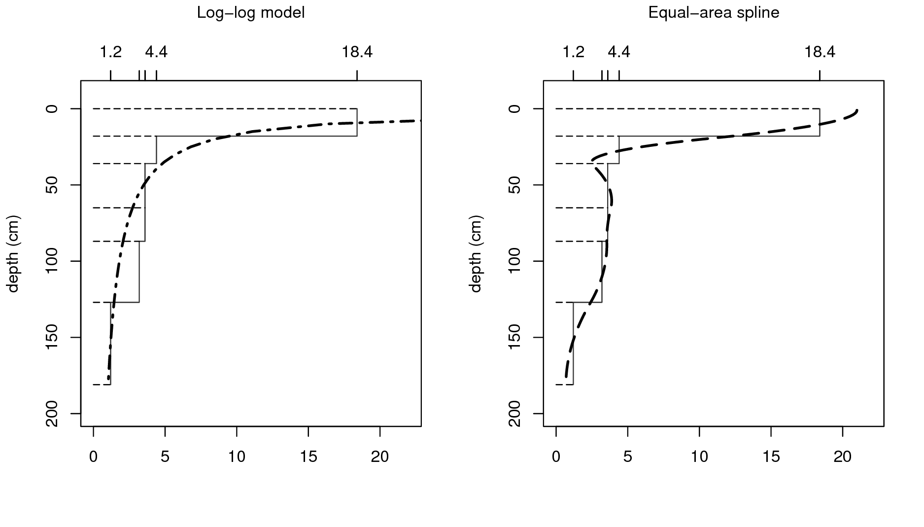
Figure 5.2: Vertical variation in soil carbon modelled using a logarithmic function (left) and a mass-preserving spline (right) with abrupt changes by horizon ilustrated with solid lines.
To fit mass preserving splines we can use:
library(aqp)
#> This is aqp 1.17
#>
#> Attaching package: 'aqp'
#> The following object is masked from 'package:base':
#>
#>     union
library(rgdal)
#> Loading required package: sp
#> rgdal: version: 1.3-6, (SVN revision 773)
#>  Geospatial Data Abstraction Library extensions to R successfully loaded
#>  Loaded GDAL runtime: GDAL 2.2.2, released 2017/09/15
#>  Path to GDAL shared files: /usr/share/gdal/2.2
#>  GDAL binary built with GEOS: TRUE
#>  Loaded PROJ.4 runtime: Rel. 4.8.0, 6 March 2012, [PJ_VERSION: 480]
#>  Path to PROJ.4 shared files: (autodetected)
#>  Linking to sp version: 1.3-1
library(GSIF)
#> GSIF version 0.5-5 (2019-01-04)
#> URL: http://gsif.r-forge.r-project.org/
#>
#> Attaching package: 'GSIF'
#> The following object is masked _by_ '.GlobalEnv':
#>
#>     munsell
prof1.spc <- prof1
depths(prof1.spc) <- id ~ top + bottom
#> Warning: converting IDs from factor to character
site(prof1.spc) <- ~ lon + lat + FAO1988
coordinates(prof1.spc) <- ~ lon + lat
proj4string(prof1.spc) <- CRS("+proj=longlat +datum=WGS84")
## fit a spline:
ORCDRC.s <- mpspline(prof1.spc, var.name="ORCDRC", show.progress=FALSE)
#> Fitting mass preserving splines per profile...
ORCDRC.s$var.std
#>   0-5 cm 5-15 cm 15-30 cm 30-60 cm 60-100 cm 100-200 cm soil depth
#> 1     21      17      7.3      3.3       3.6        1.8        181
where var.std shows average fitted values for standard depth intervals
(i.e. those given in the GlobalSoilMap specifications), and var.1cm
are the values fitted at 1–cm increments
(Fig. 5.2).
A disadvantage of using mathematical functions to convert soil observations at specific depth intervals to continuous values along the whole profile is that these values are only estimates with associated estimation errors. If estimates are treated as if these were observations then an important source of error is ignored, which may jeopardize the quality of the final soil predictions and in particular the associated uncertainty (see further section 5.3). This problem can be avoided by taking, for example, a 3D modelling approach (Poggio and Gimona 2014; Hengl, Heuvelink, et al. 2015), in which model calibration and spatial interpolation are based on the original soil observations directly (although proper use of this requires that the differences in vertical support between measurements are taken into account also). We will address this also in later sections of this chapter, among others in section 6.1.4.
5.1.4 Vertical aggregation of soil properties
As mentioned previously, soil variables refer to aggregate values over specific depth intervals (see Fig. 5.2). For example, the organic carbon content is typically observed per soil horizon with values in e.g. g/kg or permilles (Conant et al. 2010; Baritz et al. 2010; Panagos et al. 2013). The Soil Organic Carbon Storage (or Soil Organic Carbon Stock) in the whole profile can be calculated by using Eq (7.1). Once we have determined soil organic carbon storage (\(\mathtt{OCS}\)) per horizon, we can derive the total organic carbon in the soil by summing over all (\(H\)) horizons:
\[\begin{equation} \mathtt{OCS} = \sum\limits_{h = 1}^H { \mathtt{OCS}_h } \tag{5.5} \end{equation}\]Obviously, the horizon-specific soil organic carbon content (\(\mathtt{ORC}_h\)) and total soil organic carbon content (\(\mathtt{OCS}\)) are NOT the same variables and need to be analysed and mapped separately.
In the case of pH (\(\mathtt{PHI}\)) we usually do not aim at estimating the actual mass or quantity of hydrogen ions. To represent a soil profile with a single number, we may take a weighted mean of the measured pH values per horizon:
\[\begin{equation} \mathtt{PHI} = \sum\limits_{h = 1}^H { w_h \cdot \mathtt{PHI}_h }; \qquad \sum\limits_{h = 1}^H{w_h} = 1 \tag{5.6} \end{equation}\]where the weights can be chosen proportional to the horizon thickness:
\[\begin{equation} w _h = \frac{{\mathtt{HSIZE}_h}}{\sum\limits_{h = 1}^H {{\mathtt{HSIZE}}_h}} \end{equation}\]Thus, it is important to be aware that all soil variables: (A) can be expressed as relative (percentages) or absolute (mass / quantities) values, and (B) refer to specific horizons or depth intervals or to the whole soil profile.
Similar spatial support-effects show up in the horizontal, because soil observations at point locations are not the same as average or bulk soil samples taken by averaging a large number of point observations on a site or plot (Webster and Oliver 2001).
In order to avoid misinterpretation of the results of mapping, we recommend that any delivered map of soil properties should specify the support size in the vertical and lateral directions, the analysis method (detection limit) and measurement units. Such information can be included in the metadata and/or in any key visualization or plot. Likewise, any end-user of soil data should specify whether estimates of the relative or total organic carbon, aggregated or at 2D/3D point support are required.
5.2 Spatial prediction of soil variables
5.2.1 Main principles
“Pragmatically, the goal of a model is to predict, and at the same time scientists want to incorporate their understanding of how the world works into their models” (Cressie and Wikle 2011). In general terms, spatial prediction consists of the following seven steps (Fig. 5.3):
Select the target variable, scale (spatial resolution) and associated geographical region of interest;
Define a model of spatial variation for the target variable;
Prepare a sampling plan and collect samples and relevant explanatory variables;
Estimate the model parameters using the collected data;
Derive and apply the spatial prediction method associated with the selected model;
Evaluate the spatial prediction outputs and collect new data / run alternative models if necessary;
Use the outputs of the spatial prediction process for decision making and scenario testing.
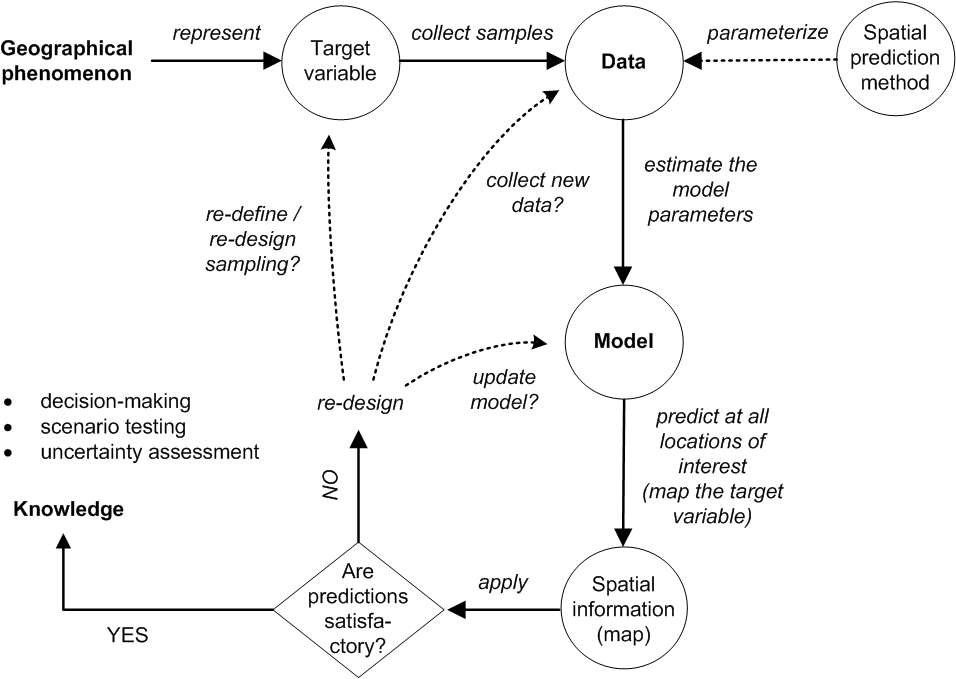
Figure 5.3: From data to knowledge and back: the general spatial prediction scheme applicable to many environmental sciences.
The spatial prediction process is repeated at all nodes of a grid covering \(D\) (or a space-time domain in case of spatiotemporal prediction) and produces three main outputs:
Estimates of the model parameters (e.g., regression coefficients and variogram parameters), i.e. the model;
Predictions at new locations, i.e. a prediction map;
Estimate of uncertainty associated with the predictions, i.e. a prediction error map.
It is clear from Fig. 5.3 that the key steps in the mapping procedure are: (a) choice of the sampling scheme (e.g. Ng et al. (2018) and Brus (2019)), (b) choice of the model of spatial variation (e.g. Diggle and Ribeiro Jr (2007)), and (c) choice of the parameter estimation technique (e.g. Lark, Cullis, and Welham (2006)). When the sampling scheme is given and cannot be changed, the focus of optimization of the spatial prediction process is then on selecting and fine-tuning the best performing spatial prediction method.
In a geostatistical framework, spatial prediction is estimation of values of some target variable \(Z\) at a new location (\({s}_0\)) given the input data:
\[\begin{equation} \hat Z({s}_0) = E\left\{ Z({s}_0)|z({s}_i), \; {{X}}({s}_0), \; i=1,...,n \right\} \tag{5.7} \end{equation}\]where the \(z({s}_i)\) are the input set of observations of the target variable, \({s}_i\) is a geographical location, \(n\) is the number of observations and \({{X}}({s}_0)\) is a list of covariates or explanatory variables, available at all prediction locations within the study area of interest (\({s} \in \mathbb{A}\)). To emphasise that the model parameters also influence the outcome of the prediction process, this can be made explicit by writing (Cressie and Wikle 2011):
\[\begin{equation} [Z|Y,{{\theta}} ] \tag{5.8} \end{equation}\]where \(Z\) is the data, \(Y\) is the (hidden) process that we are predicting, and \({{\theta}}\) is a list of model parameters e.g. trend coefficients and variogram parameters.
There are many spatial prediction methods for generating spatial
predictions from soil samples and covariate information. All differ in
the underlying statistical model of spatial variation, although this
model is not always made explicit and different methods may use the same
statistical model. A review of currently used digital soil mapping
methods is given, for example, in McBratney et al. (2011), while the most
extensive review can be found in McBratney, Mendonça Santos, and Minasny (2003) and McBratney, Minasny, and Stockmann (2018). Li and Heap (2010) list 40+ spatial prediction / spatial interpolation
techniques. Many spatial prediction methods are often
just different names for essentially the same thing.
What is often known under a single name, in the statistical,
or mathematical literature, can be implemented through
different computational frameworks, and lead to different outputs
(mainly because many models are not written out in the finest detail and leave
flexibility for actual implementation).
5.2.2 Soil sampling
A soil sample is a collection of field observations, usually represented as points. Statistical aspects of sampling methods and approaches are discussed in detail by Schabenberger and Gotway (2005) and de Gruijter et al. (2006), while some more practical suggestions for soil sampling can be found in Pansu, Gautheyrou, and Loyer (2001) Webster and Oliver (2001), Tan (2005), Legros (2006) and Brus (2019). Some general recommendations for soil sampling are:
Points need to cover the entire geographical area of interest and not overrepresent specific subareas that have much different characteristics than the main area.
Soil observations at point locations should be made using consistent measurement methods. Replicates should ideally be taken to quantify the measurement error.
Bulk sampling is recommended when short-distance spatial variation is expected to be large and not of interest to the map user.
If a variogram is to be estimated then the sample size should be >50 and there should be sufficient point pairs with small separation distances.
If trend coefficients are to be estimated then the covariates at sampling points should cover the entire feature space of each covariate.
The sampling design or rationale used to decide where to locate soil profile observations, or sampling points, is often not clear and may vary from case to case. Therefore, there is no guarantee that available legacy point data used as input to geostatistical modelling will satisfy the recommendations listed above. Many of the legacy profile data locations in the world were selected using convenience sampling. In fact, many points in traditional soil surveys may have been selected and sampled to capture information about unusual conditions or to locate boundaries at points of transition and maximum confusion about soil properties (Legros 2006). Once a soil becomes recognized as being widely distributed and dominant in the landscape, field surveyors often choose not to record observations when that soil is encountered, preferring to focus instead on recording unusual sites or areas where soil transition occurs. Thus the population of available soil point observations may not be representative of the true population of soils, with some soils being either over or under-represented.
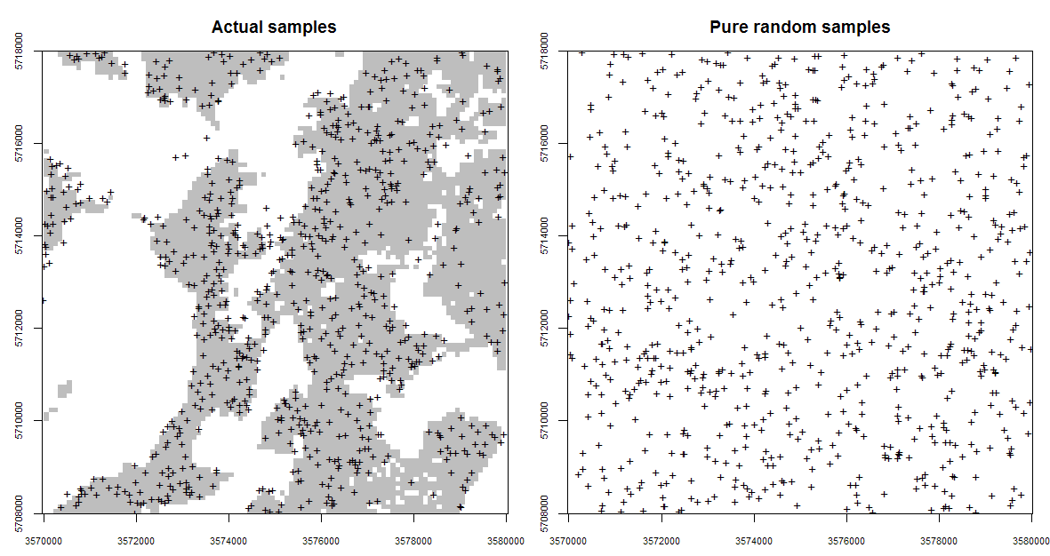
Figure 5.4: Occurrence probabilities derived for the actual sampling locations (left), and for a purely random sample design with exactly the same number of points (right). Probabilities derived using the spsample.prob function from the GSIF package. The shaded area on the left indicates which areas (in the environmental space) have been systematically represented, while the white colour indicates areas which have been systematically omitted (and which is not by chance).
Fig. 5.4 (the Ebergötzen study area) illustrates a problem of dealing with clustered samples and omission of environmental features. Using the actual samples shown in the plot on the left of Fig. 5.4 we would like to map the whole area inside the rectangle. This is technically possible, but the user should be aware that the actual Ebergötzen points systematically miss sampling some environmental features: in this case natural forests / rolling hills that were not of interest to the survey project. This does not mean that the Ebergötzen point data are not applicable for geostatistical analyses. It simply means that the sampling bias and under-representation of specific environmental conditions will lead to spatial predictions that may be biased and highly uncertain under these conditions (Brus and Heuvelink 2007).
5.2.3 Knowledge-driven soil mapping
As mentioned previously in section 1.4.8, knowledge-driven mapping is often based on unstated and unformalized rules and understanding that exists mainly in the minds and memories of the individual soil surveyors who conducted field studies and mapping. Expert, or knowledge-based, information can be converted to mapping algorithms by applying conceptual rules to decision trees and/or statistical models (MacMillan, Pettapiece, and Brierley 2005; Walter, Lagacherie, and Follain 2006; Liu and Zhu 2009). For example, a surveyor can define the classification rules subjectively, i.e. based on his/her knowledge of the area, then iteratively adjust the model until the output maps fit his/her expectation of the distribution of soils (MacMillan et al. 2010).
In areas where few, or no, field observations of soil properties are available, the most common way to produce estimates is to rely on expert knowledge, or to base estimates on data from other, similar areas. This is a kind of ‘knowledge transfer’ system. The best example of a knowledge transfer system is the concept of soil series in the USA (Simonson 1968). Soil series (+phases) are the lowest (most detailed) level classes of soil types typically mapped. Each soil series should consist of pedons having soil horizons that are similar in colour, texture, structure, pH, consistence, mineral and chemical composition, and arrangement in the soil profile.
If one finds the same type of soil series repeatedly at similar locations, then there is little need to sample the soil again at additional, similar, locations and, consequently, soil survey field costs can be reduced. This sounds like an attractive approach because one can minimize the survey costs by focusing on delineating the distribution of soil series only. The problem is that there are >15,000 soil series in the USA (Smith 1986), which obviously means that it is not easy to recognize the same soil series just by doing rapid field observations. In addition, the accuracy with which one can consistently recognize a soil series may well fail on standard kappa statistics tests, indicating that there may be substantial confusion between soil series (e.g. large measurement error).
Large parts of the world basically contain very few (sparce) field records and hence one will need to improvise to be able to produce soil predictions. One idea to map such areas is to build attribute tables for representative soil types, then map the distribution of these soil types in areas without using local field samples. Mallavan, Minasny, and McBratney (2010) refer to soil classes that can be predicted far away from the actual sampling locations as homosoils. The homosoils concept is based on the assumption that locations that share similar environments (e.g. soil-forming factors) are likely to exhibit similar soils and soil properties also.
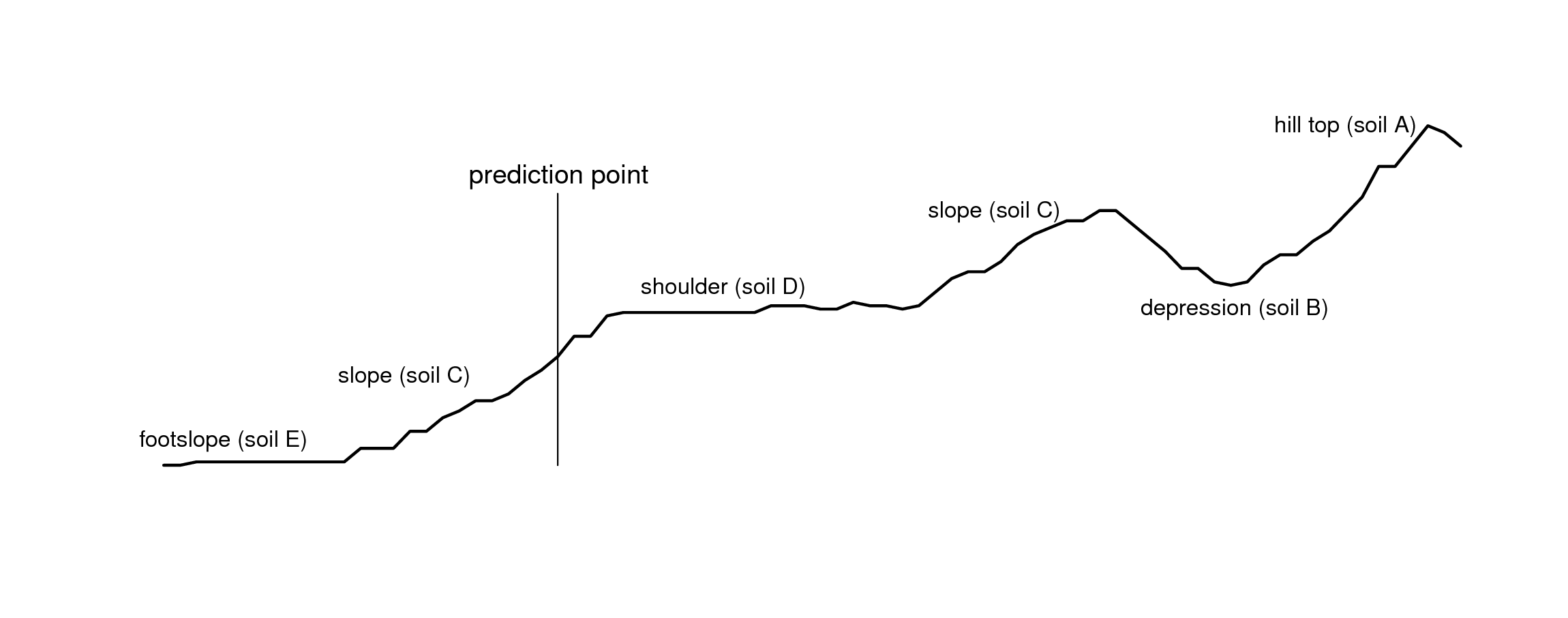
Figure 5.5: Landform positions and location of a prediction point for the Maungawhau data set.
Expert-based systems also rely on using standard mapping paradigms such as the concept of relating soil series occurrance to landscape position along a toposequence, or catena . Fig. 5.5, for example, shows a cross-section derived using the elevation data in Fig. 5.6. An experienced soil surveyor would visit the area and attempt to produce a diagram showing a sequence of soil types positioned along this cross-section. This expert knowledge can be subsequently utilized as manual mapping rules, provided that it is representative of the area, that it can be formalized through repeatable procedures and that it can be tested using real observations.
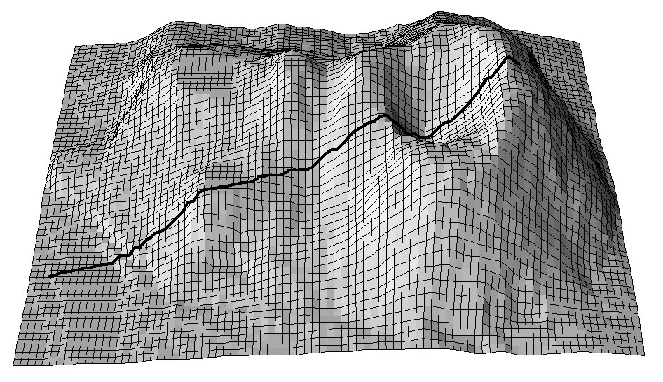
Figure 5.6: A cross-section for the Maungawhau volcano dataset commonly used in R to illustrate DEM and image analysis techniques.
If relevant auxiliary information, such as a Digital Elevation Model (DEM), is available for the study area, one can derive a number of DEM parameters that can help to quantify landforms and geomorphological processes. Landforms can also automatically be classified by computing various DEM parameters per pixel, or by using knowledge from, Fig. 5.7 (a sample of the study area) to objectively extract landforms and associated soils in an area. Such auxiliary landform information can be informative about the spatial distribution of the soil, which is the key principle of, for example, the SOTER methodology (Van Engelen and Dijkshoorn 2012).
The mapping process of knowledge-driven soil mapping can be summarized as follows (MacMillan, Pettapiece, and Brierley 2005; MacMillan et al. 2010):
Sample the study area using transects oriented along topographic cross-sections;
Assign soil types to each landform position and at each sample location;
Derive DEM parameters and other auxiliary data sets;
Develop (fuzzy) rules relating the distribution of soil classes to the auxiliary (mainly topographic) variables;
Implement (fuzzy) rules to allocate soil classes (or compute class probabi;ities) for each grid location;
Generate soil property values for each soil class using representative observations (class centers);
Estimate values of the target soil variable at each grid location using a weighted average of allocated soil class or membership values and central soil property values for each soil class;
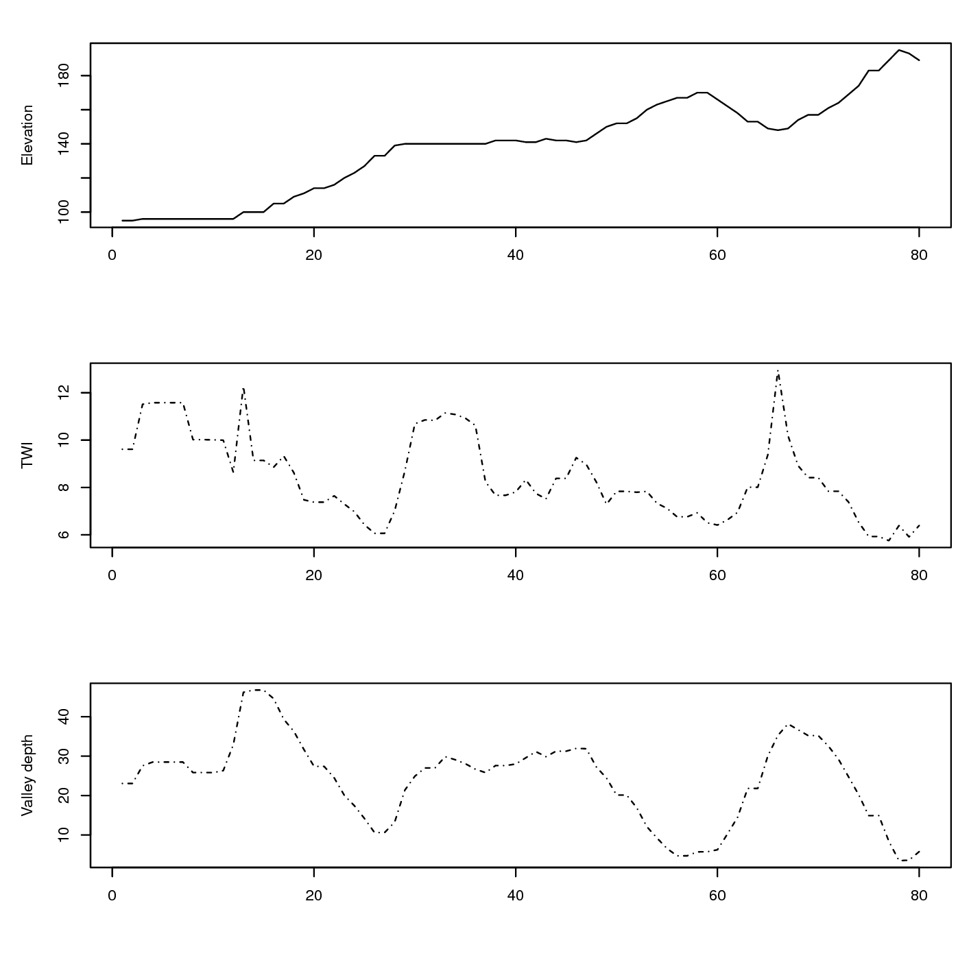
Figure 5.7: Associated values of DEM-based covariates: TWI — Topographic Wetness Index and Valley depth for the cross-section from the previous figure.
In mathematical terms, soil property prediction based on fuzzy soil classification values using the SOLIM approach Zhu et al. (2001, 2010) works as follows:
\[\begin{equation} \begin{aligned} \hat z({s}_0) = \sum\limits_{c_j = 1}^{c_p} {\nu _{c_j} ({s}_0) \cdot z_{c_j} }; & \hspace{.6cm} \sum\limits_{c_j = 1}^{c_p} {\nu _j ({s}_0)} = 1\end{aligned} \tag{5.9} \end{equation}\]where \(\hat z({s}_0)\) is the predicted soil attribute at
\({s}_0\), \(\nu _{c_j} ({s}_0)\) is the membership value of class
\(c_j\) at location \({s}_0\), and \(z_{c_j}\) is the modal (or best
representative) value of the inferred soil attribute of the \(c_j\)-th
category. The predicted soil attribute is mapped directly from
membership maps using a linear additive weighing function. Consider the
example of six soil classes A, B, C, D, E and F. The
attribute table indicates that soil type A has 10%, B 10%, C 30%,
D 40%, E 25%, and F 35% of clay. If the membership values at a
grid position are 0.6, 0.2, 0.1, 0.05, 0.00 and 0.00, then
Eq.(5.9) predicts the clay content as 13.5%.
It is obvious from this work flow that the critical aspects that determine the accuracy of the final predictions are the selection of where we locate the cross-sections and the representative soil profiles and the strength of the relationship between the resulting soil classes and target soil properties. Qi et al. (2006), for example, recommended that the most representative values for soil classes can be identified, if many soil profiles are available, by finding the sampling location that occurs at the grid cell with highest similarity value for a particular soil class. Soil mappers are now increasingly looking for ways to combine expert systems with statistical data mining and regression modelling techniques.
One problem of using a supervised mapping system, as described above, is that it is difficult to get an objective estimate of the prediction error (or at least a robust statistical theory for this has not yet been developed). The only possibility to assess the accuracy of such maps would be to collect independent validation samples and estimate the mapping accuracy following the methods described in section 5.3. So, in fact, expert-based systems also depend on statistical sampling and inference for evaluation of the accuracy of the resulting map.
5.2.4 Geostatistics-driven soil mapping (pedometric mapping)
Pedometric mapping is based on using statistical models to predict soil properties, which leads us to the field of geostatistics. Geostatistics treats the soil as a realization of a random process (Webster and Oliver 2001). It uses the point observations and gridded covariates to predict the random process at unobserved locations, which yields conditional probability distributions, whose spread (i.e. standard deviation, width of prediction intervals) explicitly characterizes the uncertainty associated with the predictions. As mentioned previously in section 1.3.6, geostatistics is a data-driven approach to soil mapping in which georeferenced point samples are the key input to map production.
Traditional geostatistics has basically been identified with various ways of variogram modeling and kriging (Haining, Kerry, and Oliver 2010). Contemporary geostatistics extends linear models and plain kriging techniques to non-linear and hybrid models; it also extends purely spatial models (2D) to 3D and space-time models (Schabenberger and Gotway 2005; Bivand, Pebesma, and Rubio 2008; Diggle and Ribeiro Jr 2007; Cressie and Wikle 2011). Implementation of more sophisticated geostatistical models for soil mapping is an ongoing activity and is quite challenging (computationally), especially in the case of fine-resolution mapping of large areas (Hengl, Mendes de Jesus, et al. 2017).
Note also that geostatistical mapping is often restricted to quantitative soil properties. Soil prediction models that predict categorical soil variables such as soil type or soil colour class are often quite complex (see e.g. Hengl, Toomanian, et al. (2007) and Kempen et al. (2009) for a discussion). Most large scale soil mapping projects also require predictions in 3D, or at least 2D predictions (layers) for several depth intervals. This can be done by treating each layer separately in a 2D analysis, possibly by taking vertical correlations into account, but also by direct 3D geostatistical modelling. Both approaches are reviewed in the following sections.
Over the last decade statisticians have recommended using model-based geostatistics as the most reliable framework for spatial predictions. The essence of model-based statistics is that “the statistical methods are derived by applying general principles of statistical inference based on an explicitly declared stochastic model of the data generating mechanism” (Diggle and Ribeiro Jr 2007; P. E. Brown 2015). This avoids ad hoc, heuristic solution methods and has the advantage that it yields generic and portable solutions. Some examples of diverse geostatistical models are given in P. E. Brown (2015).
The basic geostatistical model treats the soil property of interest as the sum of a deterministic trend and a stochastic residual:
\[\begin{equation} Z({s}) = m({s}) + \varepsilon({s}) \tag{5.10} \end{equation}\]where \(\varepsilon\) and hence \(Z\) are normally distributed stochastic processes. This is the same model as that presented in Eq.(5.1), with in this case \(\varepsilon = \varepsilon ' + \varepsilon ''\) being the sum of the spatially correlated and spatially uncorrelated stochastic components. The mean of \(\varepsilon\) is taken to be zero. Note that we use capital letter \(Z\) because we use a probabilistic model, i.e. we treat the soil property as an outcome of a stochastic process and define a model of that stochastic process. Ideally, the spatial variation of the stochastic residual of Eq.(5.10) is much less than that of the dependent variable.
When the assumption of normality is not realistic, such as when the frequency distribution of the residuals at observation locations is very skewed, the easiest solution is to take a Transformed Gaussian approach (Diggle and Ribeiro Jr 2007 ch3.8) in which the Gaussian geostatistical model is formulated for a transformation of the dependent variable (e.g. logarithmic, logit, square root, Box-Cox transform). A more advanced approach would drop the normal distribution approach entirely and assume a Generalized Linear Geostatistical Model (Diggle and Ribeiro Jr 2007; P. E. Brown 2015) but this complicates the statistical analysis and prediction process dramatically. The Transformed Gaussian approach is nearly as simple as the Gaussian approach although the back-transformation requires attention, especially when the spatial prediction includes a change of support (leading to block kriging). If this is the case, it may be necessary to use a stochastic simulation approach and derive the predictions and associated uncertainty (i.e. the conditional probability distribution) using numerical simulations.
The trend part of Eq.(5.10) (i.e. \(m\)) can take many forms. In the simplest case it would be a constant but usually it is taken as some function of known, exhaustively available covariates. This is where soil mapping can benefit from other sources of information and can implement Jenny’s State Factor Model of soil formation (Jenny, Salem, and Wallis 1968; Jenny 1994; Heuvelink and Webster 2001; McBratney et al. 2011), which has been known from the time of Dokuchaev (Florinsky 2012). The covariates are often maps of environmental properties that are known to be related to the soil property of interest (e.g. elevation, land cover, geology) but could also be the outcome of a mechanistic soil process model (such as a soil acidification model, a soil nutrient leaching model or a soil genesis model). In the case of the latter one might opt for taking \(m\) equal to the output of the deterministic model, but when the covariates are related environmental properties one must define a structure for \(m\) and introduce parameters to be estimated from paired observations of the soil property and covariates. One of the simplest approaches is to use multiple linear regression to predict values at some new location \({s}_0\) (Kutner et al. 2005):
\[\begin{equation} m({s}_0 ) = \sum\limits_{j = 0}^p { \beta _j \cdot X_j ({s}_0 )} \tag{5.11} \end{equation}\]where \(\beta _j\) are the regression model coefficients, \(\beta _0\) is the intercept, \(j=1,\ldots,p\) are covariates or explanatory variables (available at all locations within the study area of interest \(\mathbb{A}\)), and \(p\) is the number of covariates. Eq.(5.11) can also include categorical covariates (e.g. maps of land cover, geology, soil type) by representing these by as many binary dummy variables as there are categories (minus one, to be precise, since an intercept is included in the model). In addition, transformed covariates may also be included or interactions between covariates. The latter is achieved by extending the set of covariates with products or other mixtures of covariates. However, note that this will dramatically increase the number of covariates. The risk of considering a large number of covariates is that it may become difficult to obtain reliable estimates of the regression coefficients. Also one may run the risk of multicollinearity — the property of covariates being mutually strongly correlated (as indicated by Jenny, Salem, and Wallis (1968) already in (1968)).
The advantage of Eq.(5.11) is that it is linear in the unknown coefficients, which makes their estimation relatively straightforward and also permits derivation of the uncertainty about the regression coefficients (\(\beta\)). However, in many practical cases, the linear formulation may be too restrictive and that is why alternative structures have been extensively developed to establish the relationship between the dependent and covariates. Examples of these so-called ‘statistical learning’ and/or ‘machine learning’ approaches are:
artificial neural networks (Yegnanarayana 2004),
classification and regression trees (Breiman 1993),
support vector machines (Hearst et al. 1998),
computer-based expert systems,
Statistical treatment of many of these methods is given in Hastie, Tibshirani, and Friedman (2009) and Kuhn and Johnson (2013). Care needs to be taken when using machine learning techniques, such as random forest, because such techniques are more sensitive to noise and blunders in the data.
Most methods listed above require appropriate levels of expertise to avoid pitfalls and incorrect use but, when feasible and used properly, these methods should extract maximal information about the target variable from the covariates (Statnikov, Wang, and Aliferis 2008; Kanevski, Timonin, and Pozdnukhov 2009).
The trend (\(m\)) relates covariates to soil properties and for this it uses a soil-environment correlation model — the so-called CLORPT model, which was formulated by Jenny in 1941 (a (1994) reprint from that book is also available). McBratney, Mendonça Santos, and Minasny (2003) further formulated an extension of the CLORPT model known as the “SCORPAN” model.
The CLORPT model may be written as (Jenny 1994; Florinsky 2012):
\[\begin{equation} S = f (cl, o, r, p, t) \tag{5.12} \end{equation}\]where \(S\) stands for soil (properties and classes), \(cl\) for climate, \(o\) for organisms (including humans), \(r\) is relief, \(p\) is parent material or geology and \(t\) is time. In other words, we can assume that the distribution of both soil and vegetation (at least in a natural system) can be at least partially explained by environmental conditions. Eq.(5.12) suggests that soil is a result of environmental factors, while in reality there are many feedbacks and soil, in turn, influences many of the factors on the right-hand side of Eq.(5.12), such as \(cl\), \(o\) and \(r\).
Uncertainty about the estimation errors of model coefficients can fairly easily be taken into account in the subsequent prediction analysis if the model is linear in the coefficients, such as in Eq.(5.11). In this book we therefore restrict ourselves to this case but allow that the \(X_j\)’s in Eq.(5.11) are derived in various ways.
Since the stochastic residual of Eq.(5.10) is normally distributed and has zero mean, only its variance-covariance remains to be specified:
\[\begin{equation} C\left[Z({s}),Z({s}+{h})\right] = \sigma (s) \cdot \sigma(s+{h}) \cdot \rho ({h}) \end{equation}\]where \({{h}}\) is the separation distance between two locations. Note that here we assumed that the correlation function \(\rho\) is invariant to geographic translation (i.e., it only depends on the distance \({h}\) between locations and not on the locations themselves). If in addition the standard deviation \(\sigma\) would be spatially invariant then \(C\) would be second-order stationary. These type of simplifying assumptions are needed to be able to estimate the variance-covariance structure of \(C\) from the observations. If the standard deviation is allowed to vary with location, then it could be defined in a similar way as in Eq.(5.11). The correlation function \(\rho\) would be parameterised to a common form (e.g. exponential, spherical, Matérn), thus ensuring that the model is statistically valid and positive-definite. It is also quite common to assume isotropy, meaning that two-dimensional geographic distance \({{h}}\) can be reduced to one-dimensional Euclidean distance \(h\).
Once the model has been defined, its parameters must be estimated from the data. These are the regression coefficients of the trend (when applicable) and the parameters of the variance-covariance structure of the stochastic residual. Commonly used estimation methods are least squares and maximum likelihood. Both methods have been extensively described in the literature (e.g. Webster and Oliver (2001) and Diggle and Ribeiro Jr (2007)). More complex trend models may also use the same techniques to estimate their parameters, although they might also need to rely on more complex parameter estimation methods such as genetic algorithms and simulated annealing (Lark and Papritz 2003).
The optimal spatial prediction in the case of a model Eq.(5.10) with a linear trend Eq.(5.11) and a normally distributed residual is given by the well-kown Best Linear Unbiased Predictor (BLUP):
\[\begin{equation} \hat z({{{s}}_0}) = {{X}}_{{0}}^{{T}}\cdot \hat{{\beta}} + \hat{{\lambda}}_{{0}}^{{T}}\cdot({{z}} - {{X}}\cdot \hat{{\beta}} ) \tag{5.13} \end{equation}\]where the regression coefficients and kriging weights are estimated using:
\[\begin{equation} \begin{aligned} \hat{{\beta}} &= {\left( {{{{X}}^{{T}}}\cdot{{{C}}^{ - {{1}}}}\cdot{{X}}} \right)^{ - {{1}}}}\cdot{{{X}}^{{T}}}\cdot{{{C}}^{ - {{1}}}}\cdot{{z}} \\ \hat{{\lambda}}_{{0}} &= {C}^{ - {{1}}} \cdot {{c}}_{{0}} \notag\end{aligned} \tag{5.14} \end{equation}\]and where \({{X}}\) is the matrix of \(p\) predictors at the \(n\) sampling locations, \(\hat{{\beta}}\) is the vector of estimated regression coefficients, \({C}\) is the \(n\)\(n\) variance-covariance matrix of residuals, \({c}_{{0}}\) is the vector of \(n\)\(1\) covariances at the prediction location, and \({\lambda}_{{0}}\) is the vector of \(n\) kriging weights used to interpolate the residuals. Derivation of BLUP for spatial data can be found in many standard statistical books e.g. Stein (1999), Christensen (2001, 277), Venables and Ripley (2002, 425–30) and/or Schabenberger and Gotway (2005).
Any form of kriging computes the conditional distribution of \(Z({{s}}_0)\) at an unobserved location \({{s}}_0\) from the observations \(z({{s}}_1 )\), \(z({{s}}_2 ), \ldots , z({{s}}_n )\) and the covariates \({{X}}({{s}}_0)\) (matrix of size \(p \times n\)). From a statistical perspective this is straightforward for the case of a linear model and normally distributed residuals. However, solving large matrices and more sophisticated model fitting algorithms such as restricted maximum likelihood can take a significant amount of time if the number of observations is large and/or the prediction grid dense. Pragmatic approaches to addressing constraints imposed by large data sets are to constrain the observation data set to local neighbourhoods or to take a multiscale nested approach.
Kriging not only yields optimal predictions but also quantifies the prediction error with the kriging standard deviation. Prediction intervals can be computed easily because the prediction errors are normally distributed. Alternatively, uncertainty in spatial predictions can also be quantified with spatial stochastic simulation. While kriging yields the ‘optimal’ prediction of the soil property at any one location, spatial stochastic simulation yields a series of possible values by sampling from the conditional probability distribution. In this way a large number of ‘realizations’ can be generated, which can be useful when the resulting map needs to be back-transformed or when it is used in a spatial uncertainty propagation analysis. Spatial stochastic simulation of the linear Gaussian model can be done using a technique known as sequential Gaussian simulation (Goovaerts 1997; Yamamoto 2008). It is not, in principal, more difficult than kriging but it is certainly numerically more demanding i.e. takes significantly more time to compute.
5.2.5 Regression-kriging (generic model)
Ignoring the assumptions about the cross-correlation between the trend and residual components, we can extend the regression-kriging model and use any type of (non-linear) regression to predict values ( e.g. regression trees, artificial neural networks and other machine learning models), calculate residuals at observation locations, fit a variogram for these residuals, interpolate the residuals using ordinary or simple kriging, and add the result to the predicted regression part. This means that RK can, in general, be formulated as:
\[\begin{equation} {\rm prediction} \; = \; \begin{matrix} {\rm trend} \; {\rm predicted} \\ {\rm using} \; {\rm regression} \end{matrix} \; + \; \begin{matrix} {\rm residual} \; {\rm predicted} \\ {\rm using} \; {\rm kriging} \end{matrix} \tag{5.15} \end{equation}\]Again, statistical inference and prediction is relatively simple if the stochastic residual, or a transformation thereof, may be assumed normally distributed. Error of the regression-kriging model is likewise a sum of the regression and the kriging model errors.
5.2.6 Spatial Prediction using multiple linear regression
The predictor \(\hat Y({{ s}_0})\) of \(Y({{ s}_0})\) is typically taken as a function of covariates and the \(Y({ s}_i)\) which, upon substitution of the observations \(y({ s}_i)\), yields a (deterministic) prediction \(\hat y({{ s}_0})\). In the case of multiple linear regression (MLR), model assumptions state that at any location in \(D\) the dependent variable is the sum of a linear combination of the covariates at that location and a zero-mean normally distributed residual. Thus, at the \(n\) observation locations we have:
\[\begin{equation} { Y} = { X}^{{ T}} \cdot { \beta} + { \varepsilon} \tag{5.16} \end{equation}\]where \({ Y}\) is a vector of the target variable at the \(n\) observation locations, \({ X}\) is an \(n \times p\) matrix of covariates at the same locations and \({ \beta}\) is a vector of \(p\) regression coefficients. The stochastic residual \({ \varepsilon}\) is assumed to be independently and identically distributed. The paired observations of the target variable and covariates (\({ y}\) and \({ X}\)) are used to estimate the regression coefficients using, e.g., Ordinary Least Squares (Kutner et al. 2004):
\[\begin{equation} \hat{{ \beta}} = \left( {{{ X}}^{{ T}} \cdot {{ X}}} \right)^{ - {{ 1}}} \cdot {{ X}}^{{ T}} \cdot {{ y}} \tag{5.17} \end{equation}\]once the coefficients are estimated, these can be used to generate a prediction at \({ s}_0\):
\[\begin{equation} \hat y({ s}_0) = { x}_0^{ T} \cdot { \hat \beta} \end{equation}\]with associated prediction error variance:
\[\begin{equation} \sigma ^2 ({ s}_0 ) = var\left[ \varepsilon ({ s}_0) \right] \cdot \left[ {1 + {\mathbf x}_0^{\rm T} \cdot \left( {{\mathbf X}^{\rm T} \cdot {\mathbf X}} \right)^{ - {\mathbf 1}} \cdot {\mathbf x}_0 } \right] \tag{5.18} \end{equation}\]here, \({\mathbf x}_0\) is a vector with covariates at the prediction location and \(var\left[ \varepsilon ({ s}_0) \right]\) is the variance of the stochastic residual. The latter is usually estimated by the mean squared error (MSE):
\[\begin{equation} {\mathrm{MSE}} = \frac{\sum\limits_{i = 1}^n {(y_i - \hat y_i)^2}}{n-p} \end{equation}\]The prediction error variance given by Eq.(5.18) is smallest at prediction points where the covariate values are in the center of the covariate (‘feature’) space and increases as predictions are made further away from the center. They are particularly large in case of extrapolation in feature space (Kutner et al. 2004). Note that the model defined in Eq.(5.16) is a non-spatial model because the observation locations and spatial-autocorrelation of the dependent variable are not taken into account.
5.2.7 Universal kriging prediction error
In the case of universal kriging, regression-kriging or Kriging with External Drift, the prediction error is computed as (Christensen 2001):
\[\begin{equation} \hat \sigma _{\tt{UK}}^2 ({{s}}_0 ) = (C_0 + C_1 ) - {{c}}_{{0}}^{{T}} \cdot {{C}}^{ - {{1}}} \cdot {{c}}_{{0}} + \theta_0 \tag{5.19} \end{equation}\] \[\begin{equation} \theta_0 = \left( {{{X}}_{{0}} - {{X}}^{{T}} \cdot {{C}}^{ - {{1}}} \cdot {{c}}_{{0}} } \right)^{{T}} \cdot \left( {{{X}}^{{T}} \cdot {{C}}^{ - {{1}}} \cdot {{X}}} \right)^{{{ - 1}}} \cdot \left( {{{X}}_{{0}} - {{X}}^{{T}} \cdot {{C}}^{ - {{1}}} \cdot {{c}}_{{0}} } \right) \tag{5.20} \end{equation}\]where \(C_0 + C_1\) is the sill variation (variogram parameters), \({C}\) is the covariance matrix of the residuals, and \({{c}}_0\) is the vector of covariances of residuals at the unvisited location.
Ignoring the mixed component of the prediction variance in Eq.(5.20), one can also derive a simplified regression-kriging variance i.e. as a sum of the kriging variance and the standard error of estimating the regression mean:
\[\begin{equation} \hat \sigma _{\tt{RK}}^2 ({{s}}_0) = (C_0 + C_1 ) - {{c}}_{{0}}^{{T}} \cdot {{C}}^{ - {{1}}} \cdot {{c}}_{{0}} + {\it{SEM}}^2 \tag{5.21} \end{equation}\]Note that there will always be a small difference between results of Eq.(5.19) and Eq.(5.21), and this is a major disadvantage of using the general regression-kriging framework for spatial prediction. Although the predicted mean derived by using regression-kriging or universal kriging approaches might not differ, the estimate of the prediction variance using Eq.(5.21) will be suboptimal as it ignores product component. On the other hand, the advantage of running separate regression and kriging predictions is often worth the sacrifice as the computing time is an order of magnitude shorter and we have more flexibility to combine different types of regression models with kriging when regression is run separately from kriging (Hengl, Heuvelink, and Rossiter 2007).
5.2.8 Regression-kriging examples
The type of regression-kriging model explained in the previous section can be implemented here by combining the regression and geostatistics packages. Consider for example the Meuse case study:
library(gstat)
demo(meuse, echo=FALSE)
We can overlay the points and grids to create the regression matrix by:
meuse.ov <- over(meuse, meuse.grid)
meuse.ov <- cbind(as.data.frame(meuse), meuse.ov)
head(meuse.ov[,c("x","y","dist","soil","om")])
#>        x      y   dist soil   om
#> 1 181072 333611 0.0014    1 13.6
#> 2 181025 333558 0.0122    1 14.0
#> 3 181165 333537 0.1030    1 13.0
#> 4 181298 333484 0.1901    2  8.0
#> 5 181307 333330 0.2771    2  8.7
#> 6 181390 333260 0.3641    2  7.8
which lets us fit a linear model for organic carbon as a function of distance to river and soil type:
m <- lm(log1p(om)~dist+soil, meuse.ov)
summary(m)
#>
#> Call:
#> lm(formula = log1p(om) ~ dist + soil, data = meuse.ov)
#>
#> Residuals:
#>     Min      1Q  Median      3Q     Max
#> -1.0831 -0.1504  0.0104  0.2098  0.5913
#>
#> Coefficients:
#>             Estimate Std. Error t value  Pr(>|t|)
#> (Intercept)   2.3421     0.0425   55.05   < 2e-16 ***
#> dist         -0.8009     0.1787   -4.48 0.0000147 ***
#> soil2        -0.3358     0.0702   -4.78 0.0000041 ***
#> soil3         0.0366     0.1247    0.29      0.77
#> ---
#> Signif. codes:  0 '***' 0.001 '**' 0.01 '*' 0.05 '.' 0.1 ' ' 1
#>
#> Residual standard error: 0.33 on 149 degrees of freedom
#>   (2 observations deleted due to missingness)
#> Multiple R-squared:  0.384,  Adjusted R-squared:  0.371
#> F-statistic: 30.9 on 3 and 149 DF,  p-value: 1.32e-15
Next, we can derive the regression residuals and fit a variogram:
meuse.s <- meuse[-m$na.action,]
meuse.s$om.res <- resid(m)
vr.fit <- fit.variogram(variogram(om.res~1, meuse.s), vgm(1, "Exp", 300, 1))
vr.fit
#>   model psill range
#> 1   Nug 0.048     0
#> 2   Exp 0.065   285
With this, all model parameters (four regression coefficients and three variogram parameters) for regression-kriging have been estimated and the model can be used to generate predictions. Note that the regression model we fitted is significant, and the remaining residuals still show spatial auto-correlation. The nugget variation is about 1/3rd of the sill variation.
Using the gstat package (Pebesma 2004; Bivand, Pebesma, and Rubio 2013), regression and kriging can be combined by running universal kriging or kriging with external drift (Hengl, Heuvelink, and Rossiter 2007). First, the variogram of the residuals is calculated:
v.s <- variogram(log1p(om)~dist+soil, meuse.s)
vr.fit <- fit.variogram(v.s, vgm(1, "Exp", 300, 1))
vr.fit
#>   model psill range
#> 1   Nug 0.048     0
#> 2   Exp 0.065   285
which gives almost the same model parameter values as the
regression-kriging above. Next, the kriging can be executed with a
single call to the generic krige function:
om.rk <- krige(log1p(om)~dist+soil, meuse.s, meuse.grid, vr.fit)
#> [using universal kriging]
The package nlme fits the regression model and the variogram of the residuals concurrently (Pinheiro and Bates 2009):
library(nlme)
m.gls <- gls(log1p(om)~dist+soil, meuse.s, correlation=corExp(nugget=TRUE))
m.gls
#> Generalized least squares fit by REML
#>   Model: log1p(om) ~ dist + soil
#>   Data: meuse.s
#>   Log-restricted-likelihood: -26
#>
#> Coefficients:
#> (Intercept)        dist       soil2       soil3
#>       2.281      -0.623      -0.244      -0.057
#>
#> Correlation Structure: Exponential spatial correlation
#>  Formula: ~1
#>  Parameter estimate(s):
#>  range nugget
#>   2.00   0.07
#> Degrees of freedom: 153 total; 149 residual
#> Residual standard error: 0.34
In this case, the regression coefficients have been estimated using Eq.(5.14) i.e. via Restricted maximum likelihood (REML). The advantage of fitting the regression model and spatial autocorrelation structure concurrently is that both fits are adjusted: the estimation of the regression coefficients is adjusted for spatial autocorrelation of the residual and the variogram parameters are adjusted for the adjusted trend estimate. A disadvantage of using the nlme package is that the computational intensity increases with the size of the data set, so for any data set >1000 points the computation time can increase to tens of hours of computing. On the other hand, coefficients fitted by REML methods might not result in significantly better predictions. Getting the most objective estimate of the model parameters is sometimes not worth the effort, as demonstrated by Minasny and McBratney (2007).
Simultaneous estimation of regression coefficients and variogram parameters and including estimation errors in regression coefficients into account by using universal kriging / kriging with external drift is more elegant from a statistical point of view, but there are computational and other challenges. One of these is that it is difficult to implement global estimation of regression coefficients with local spatial prediction of residuals, which is a requirement in the case of large spatial data sets. Also, the approach does not extend to more complex non-linear trend models. In such cases, we recommend separating trend estimation from kriging of residuals by using the regression-kriging approach discussed above (Eq.(5.15)).
5.2.9 Regression-kriging examples using the GSIF package
In the GSIF package, most of the steps described above (regression modelling and variogram modelling) used to fit regression-kriging models are wrapped into generic functions. A regression-kriging model can be fitted in one step by running:
omm <- fit.gstatModel(meuse, log1p(om)~dist+soil, meuse.grid)
#> Fitting a linear model...
#> Fitting a 2D variogram...
#> Saving an object of class 'gstatModel'...
str(omm, max.level = 2)
#> Formal class 'gstatModel' [package "GSIF"] with 4 slots
#>   ..@ regModel :List of 32
#>   .. ..- attr(*, "class")= chr [1:2] "glm" "lm"
#>   ..@ vgmModel :'data.frame':    2 obs. of  9 variables:
#>   .. ..- attr(*, "singular")= logi FALSE
#>   .. ..- attr(*, "SSErr")= num 0.00000107
#>   .. ..- attr(*, "call")= language gstat::fit.variogram(object = svgm, model = ivgm)
#>   ..@ svgmModel:'data.frame':    15 obs. of  6 variables:
#>   .. ..- attr(*, "direct")='data.frame': 1 obs. of  2 variables:
#>   .. ..- attr(*, "boundaries")= num [1:16] 0 106 213 319 426 ...
#>   .. ..- attr(*, "pseudo")= num 0
#>   .. ..- attr(*, "what")= chr "semivariance"
#>   ..@ sp       :Formal class 'SpatialPointsDataFrame' [package "sp"] with 5 slots
the resulting gstatModel class object consists of a (1) regression
component, (2) variogram model for residual, and (3) sample variogram
for plotting, (4) spatial locations of observations used to fit the model. To predict values of organic carbon using this model, we can run:
om.rk <- predict(omm, meuse.grid)
#> Subsetting observations to fit the prediction domain in 2D...
#> Generating predictions using the trend model (RK method)...
#> [using ordinary kriging]
#>
100% done
#> Running 5-fold cross validation using 'krige.cv'...
#> Creating an object of class "SpatialPredictions"
om.rk
#>   Variable           : om
#>   Minium value       : 1
#>   Maximum value      : 17
#>   Size               : 153
#>   Total area         : 4964800
#>   Total area (units) : square-m
#>   Resolution (x)     : 40
#>   Resolution (y)     : 40
#>   Resolution (units) : m
#>   GLM call formula   : log1p(om) ~ dist + soil
#>   Family             : gaussian
#>   Link function      : identity
#>   Vgm model          : Exp
#>   Nugget (residual)  : 0.048
#>   Sill (residual)    : 0.065
#>   Range (residual)   : 285
#>   RMSE (validation)  : 2.4
#>   Var explained      : 49.4%
#>   Effective bytes    : 295
#>   Compression method : gzip
## back-transformation:
meuse.grid$om.rk <- expm1(om.rk@predicted$om + om.rk@predicted$var1.var/2)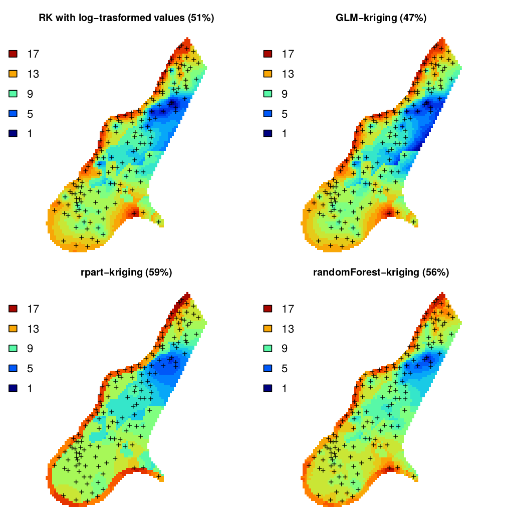
Figure 5.8: Predictions of organic carbon in percent (top soil) for the Meuse data set derived using regression-kriging with transformed values, GLM-kriging, regression tress (rpart) and random forest models combined with kriging. The percentages in brackets indicates amount of variation explained by the models.
We could also have opted for fitting a GLM with a link function, which would look like this:
omm2 <- fit.gstatModel(meuse, om~dist+soil, meuse.grid, family=gaussian(link=log))
#> Fitting a linear model...
#> Fitting a 2D variogram...
#> Saving an object of class 'gstatModel'...
summary(omm2@regModel)
#>
#> Call:
#> glm(formula = om ~ dist + soil, family = fit.family, data = rmatrix)
#>
#> Deviance Residuals:
#>    Min      1Q  Median      3Q     Max
#> -7.066  -1.492  -0.281   1.635   7.401
#>
#> Coefficients:
#>             Estimate Std. Error t value Pr(>|t|)
#> (Intercept)   10.054      0.348   28.88  < 2e-16 ***
#> dist          -8.465      1.461   -5.79    4e-08 ***
#> soil2         -2.079      0.575   -3.62  0.00041 ***
#> soil3          0.708      1.021    0.69  0.48913
#> ---
#> Signif. codes:  0 '***' 0.001 '**' 0.01 '*' 0.05 '.' 0.1 ' ' 1
#>
#> (Dispersion parameter for gaussian family taken to be 7.2)
#>
#>     Null deviance: 1791.4  on 152  degrees of freedom
#> Residual deviance: 1075.5  on 149  degrees of freedom
#>   (2 observations deleted due to missingness)
#> AIC: 742.6
#>
#> Number of Fisher Scoring iterations: 2
om.rk2 <- predict(omm2, meuse.grid)
#> Subsetting observations to fit the prediction domain in 2D...
#> Generating predictions using the trend model (RK method)...
#> [using ordinary kriging]
#>
100% done
#> Running 5-fold cross validation using 'krige.cv'...
#> Creating an object of class "SpatialPredictions"
or fitting a regression tree:
omm3 <- fit.gstatModel(meuse, log1p(om)~dist+soil, meuse.grid, method="rpart")
#> Fitting a regression tree model...
#> Estimated Complexity Parameter (for prunning): 0.09396
#> Fitting a 2D variogram...
#> Saving an object of class 'gstatModel'...
or a random forest model:
omm4 <- fit.gstatModel(meuse, om~dist+soil, meuse.grid, method="quantregForest")
#> Fitting a Quantile Regression Forest model...
#> Fitting a 2D variogram...
#> Saving an object of class 'gstatModel'...
All regression-kriging models listed above are valid and the differences between their respective results are not likely to be large (Fig. 5.8). Regression tree combined with kriging (rpart-kriging) seems to produce slightly better results i.e. smallest cross-validation error, although the difference between the four prediction methods is, in fact, not large (±5% of variance explained). It is important to run such comparisons nevertheless, as they allow us to objectively select the most efficient method.
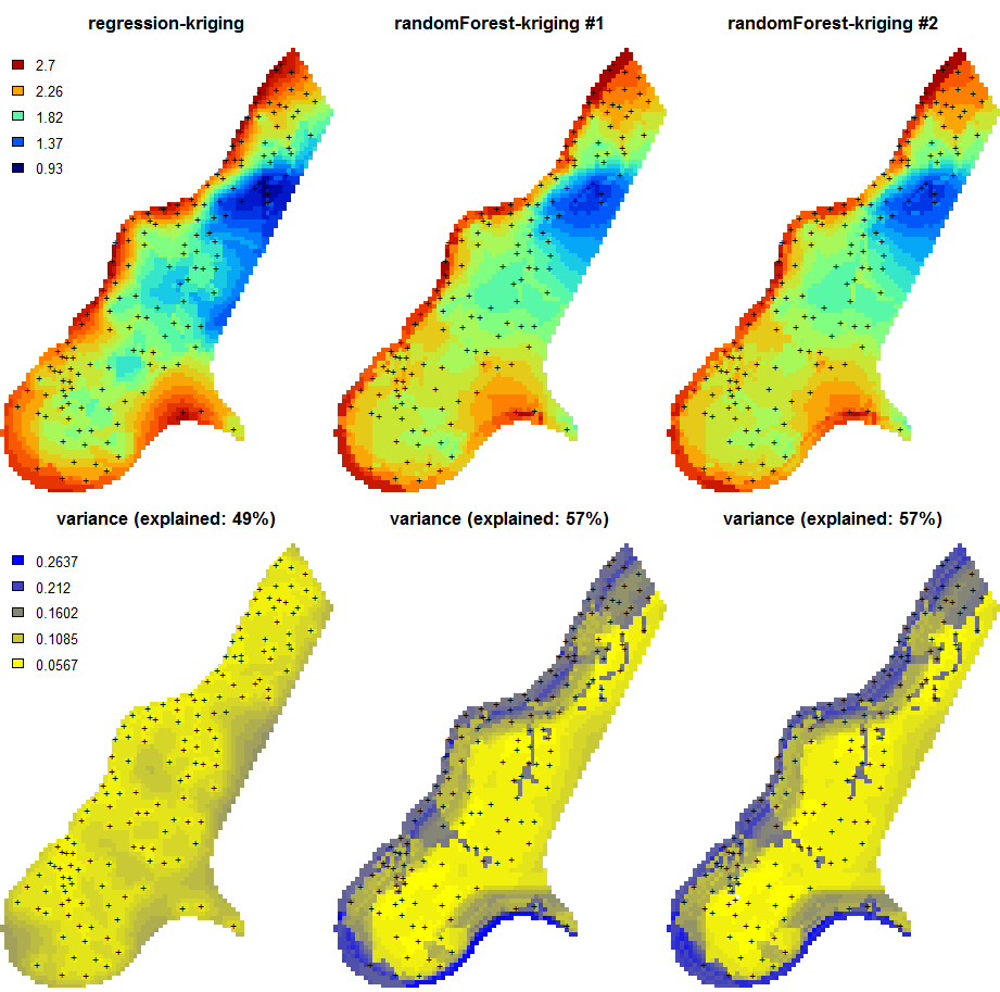
Figure 5.9: Predictions of the organic carbon (log-transformed values) using random forest vs linear regression-kriging. The random forest-kriging variance has been derived using the quantregForest package.
Fig. 5.9 shows the RK variance derived for the random forest model using the quantregForest package (Meinshausen 2006) and the formula in Eq.(5.21). Note that the quantregForest package estimates a much larger prediction variance than simple linear RK for large parts of the study area.
5.2.10 Regression-kriging and polygon averaging
Although many soil mappers may not realize it, many simpler regression-based techniques can be viewed as a special case of RK, or its variants. Consider for example a technique commonly used to generate predictions of soil properties from polygon maps: weighted averaging. Here the principal covariate available is a polygon map (showing the distribution of mapping units). In this model it is assumed that the trend is constant within mapping units and that the stochastic residual is spatially uncorrelated. In that case, the Best Linear Unbiased Predictor of the values is simple averaging of soil properties per unit (Webster and Oliver 2001, 43):
\[\begin{equation} \hat z({{s}}_0 ) = \bar \mu _p = \frac{1}{{n_p }}\sum\limits_{i = 1}^{n_p } {z({{s}}_i )} \tag{5.22} \end{equation}\]The output map produced by polygon averaging will exhibit abrupt changes at boundaries between polygon units. The prediction variance of this area-class prediction model is simply the sum of the within-unit variance and the estimation variance of the unit mean:
\[\begin{equation} \hat \sigma^2 ({{s}}_0 ) = \left( 1 + \frac{1}{n_p } \right) \cdot \sigma _p^2 \tag{5.23} \end{equation}\]From Eq.(5.23), it is evident that the accuracy of the prediction under this model depends on the degree of within-unit variation. The approach is advantageous if the within-unit variation is small compared to the between-unit variation. The predictions under this model can also be expressed as:
\[\begin{equation} \hat z({{s}}_0 ) = \sum\limits_{i = 1}^n {w_i \cdot z({{s}}_i)}; \qquad w_i = \left\{ {\begin{array}{*{20}c} {1/n_p } & {{\rm for} \; {{s}}_i \in p} \\ 0 & {{\rm otherwise}} \\ \end{array} } \right. \end{equation}\]where \(p\) is the unit identifier. So, in fact, weighted averaging per unit is a special version of regression-kriging where spatial autocorrelation is ignored (assumed zero) and all covariates are categorical variables.
Going back to the Meuse data set, we can fit a regression model for organic matter using soil types as predictors, which gives:
omm <- fit.gstatModel(meuse, log1p(om)~soil-1, meuse.grid)
#> Fitting a linear model...
#> Fitting a 2D variogram...
#> Saving an object of class 'gstatModel'...
summary(omm@regModel)
#>
#> Call:
#> glm(formula = log1p(om) ~ soil - 1, family = fit.family, data = rmatrix)
#>
#> Deviance Residuals:
#>     Min       1Q   Median       3Q      Max
#> -1.0297  -0.2087  -0.0044   0.2098   0.6668
#>
#> Coefficients:
#>       Estimate Std. Error t value Pr(>|t|)
#> soil1   2.2236     0.0354    62.9   <2e-16 ***
#> soil2   1.7217     0.0525    32.8   <2e-16 ***
#> soil3   1.9293     0.1006    19.2   <2e-16 ***
#> ---
#> Signif. codes:  0 '***' 0.001 '**' 0.01 '*' 0.05 '.' 0.1 ' ' 1
#>
#> (Dispersion parameter for gaussian family taken to be 0.12)
#>
#>     Null deviance: 672.901  on 153  degrees of freedom
#> Residual deviance:  18.214  on 150  degrees of freedom
#>   (2 observations deleted due to missingness)
#> AIC: 116.6
#>
#> Number of Fisher Scoring iterations: 2
and these regression coefficients for soil classes 1, 2, 3 are
equal to the mean values per class:
aggregate(log1p(om) ~ soil, meuse, mean)
#>   soil log1p(om)
#> 1    1       2.2
#> 2    2       1.7
#> 3    3       1.9
Note that this equality can be observed only if we remove the intercept from the regression model, hence we use:
log1p(om) ~ soil-1and NOT:
log1p(om) ~ soilThe RK model can also be extended to fuzzy memberships, in which case \({\rm{MU}}\) values are binary variables with continuous values in the range 0–1. Hence also the SOLIM model Eq.(5.9) is in fact just a special version of regression on mapping units:
\[\begin{equation} \hat z({{s}}_0 ) = \sum\limits_{c_j = 1}^{c_p} {\nu _{c_j} ({{s}}_0) \cdot z_{c_j} } = \sum\limits_{j = 1}^p { {\rm{MU}}_j \cdot \hat b_j} \hspace{.5cm} {\rm {for}} \hspace{.5cm} z_{c_j} = \frac{1}{{n_p }}\sum\limits_{i = 1}^{n_p } {z({{s}}_i )} \tag{5.24} \end{equation}\]where \({\rm{MU}}\) is the mapping unit or soil type, \(z_{c_j}\) is the modal (or most representative) value of some soil property \(z\) for the \(c_j\) class, and \(n_p\) is total number of points in some mapping unit \({\rm{MU}}\).
Ultimately, spatially weighted averaging of values per mapping unit, different types of regression, and regression kriging are all, in principle, different variants of the same statistical method. The differences are related to whether only categorical or both categorical and continuous covariates are used and whether the stochastic residual is spatially correlated or not. Although there are different ways to implement combined deterministic/stochastic predictions, one should not treat these nominally equivalent techniques as highly different.
5.2.11 Predictions at point vs block support
The geostatistical model refers to a soil variable that is defined by
the type of property and how it is measured (e.g. soil pH (KCl), soil pH
(H\(_2\)O), clay content, soil organic carbon measured with spectroscopy),
but also to the size and orientation of the soil samples that were taken
from the field. This is important because the spatial variation of the
dependent variable strongly depends on the support size (e.g. due to an
averaging out effect, the average organic content of bulked samples taken
from 1 ha plots typically has less spatial variation than that of single
soil samples taken from squares). This implies that observations at
different supports cannot be merged without taking this effect into
account (Webster and Oliver 2001). When making spatial predictions using
kriging one can use block-kriging (Webster and Oliver 2001) or
area-to-point kriging (Kyriakidis 2004) to make predictions at
larger or smaller supports. Both block-kriging and area-to-point kriging
are implemented in the gstat package via the generic function krige (Pebesma 2004).
Support can be defined as the integration volume or aggregation level at which an observation is taken or for which an estimate or prediction is given. Support is often used in the literature as a synonym for scale — large support can be related to coarse or general scales and vice versa (Hengl 2006). The notion of support is important to characterize and relate different scales of soil variation (Schabenberger and Gotway 2005). Any research of soil properties is made with specific support and spatial spacing, the latter being the distance between sampling locations. If properties are to be used with different support, e.g. when model inputs require a different support than the support of the observations, scaling (aggregation or disaggregation) becomes necessary (Heuvelink and Pebesma 1999).
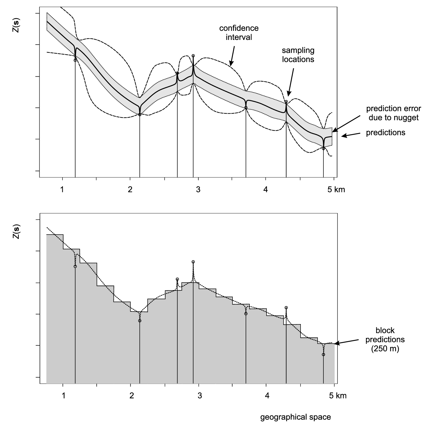
Figure 5.10: Scheme with predictions on point (above) and block support (below). In the case of various versions of kriging, both point and block predictions smooth the original measurements proportionally to the nugget variation. After Goovaerts (1997).
Depending on how significant the nugget variation is, prediction variance estimated by a model can be significantly reduced by increasing the support from points to blocks. The block kriging variance is smaller than the point kriging variance for an amount approximately equal to the nugget variation. Even if we take a block size of a few meters this decreases the prediction error significantly, if indeed the nugget variation occurs within a few meters. Because, by definition, many kriging-type techniques smooth original sampled values, one can easily notice that for support sizes smaller than half of the average shortest distance between the sampling locations, both point and block predictions might lead to practically the same predictions (see some examples by Goovaerts (1997, 158), Heuvelink and Pebesma (1999) and/or Hengl (2006)).
Consider, for example, point and block predictions and simulations using the estimates of organic matter content in the topsoil (in dg/kg) for the Meuse case study. We first generate predictions and simulations on point support:
omm <- fit.gstatModel(meuse, log1p(om)~dist+soil, meuse.grid)
#> Fitting a linear model...
#> Fitting a 2D variogram...
#> Saving an object of class 'gstatModel'...
om.rk.p <- predict(omm, meuse.grid, block=c(0,0))
#> Subsetting observations to fit the prediction domain in 2D...
#> Generating predictions using the trend model (RK method)...
#> [using ordinary kriging]
#>
100% done
#> Running 5-fold cross validation using 'krige.cv'...
#> Creating an object of class "SpatialPredictions"
om.rksim.p <- predict(omm, meuse.grid, nsim=20, block=c(0,0))
#> Subsetting observations to fit the prediction domain in 2D...
#> Generating 20 conditional simulations using the trend model (RK method)...
#> drawing 20 GLS realisations of beta...
#> [using conditional Gaussian simulation]
#>
100% done
#> Creating an object of class "RasterBrickSimulations"
#> Loading required package: raster
#>
#> Attaching package: 'raster'
#> The following object is masked from 'package:nlme':
#>
#>     getData
#> The following objects are masked from 'package:aqp':
#>
#>     metadata, metadata<-
where the argument block defines the support size for the predictions
(in this case points). To produce predictions on block support for
square blocks of 40 by 40 m we run:
om.rk.b <- predict(omm, meuse.grid, block=c(40,40), nfold=0)
#> Subsetting observations to fit the prediction domain in 2D...
#> Generating predictions using the trend model (RK method)...
#> [using ordinary kriging]
#>
100% done
#> Creating an object of class "SpatialPredictions"
om.rksim.b <- predict(omm, meuse.grid, nsim=2, block=c(40,40), debug.level=0)
#> Subsetting observations to fit the prediction domain in 2D...
#> Generating 2 conditional simulations using the trend model (RK method)...
#> Creating an object of class "RasterBrickSimulations"
## computationally intensive
Visual comparison confirms that the point and block kriging prediction maps are quite similar, while the block kriging variance is much smaller than the point kriging variance (Fig. 5.11).
Even though block kriging variances are smaller than point kriging
variances this does not imply that block kriging should always be
preferred over point kriging. If the user interest is in point values
rather than block averages, point kriging should be used. Block kriging
is also computationally more demanding than point kriging. Note also
that it is more difficult (read: more expensive) to validate block
kriging maps. In the case of point predictions, maps can be validated to
some degree using cross-validation, which is inexpensive. For example,
via one can estimate the cross-validation error using the krige.cv
function. The gstat package reports automatically the cross-validation error
(Hengl, Nikolić, and MacMillan 2013):
om.rk.p
#>   Variable           : om
#>   Minium value       : 1
#>   Maximum value      : 17
#>   Size               : 153
#>   Total area         : 4964800
#>   Total area (units) : square-m
#>   Resolution (x)     : 40
#>   Resolution (y)     : 40
#>   Resolution (units) : m
#>   GLM call formula   : log1p(om) ~ dist + soil
#>   Family             : gaussian
#>   Link function      : identity
#>   Vgm model          : Exp
#>   Nugget (residual)  : 0.048
#>   Sill (residual)    : 0.065
#>   Range (residual)   : 285
#>   RMSE (validation)  : 2.5
#>   Var explained      : 47.3%
#>   Effective bytes    : 313
#>   Compression method : gzip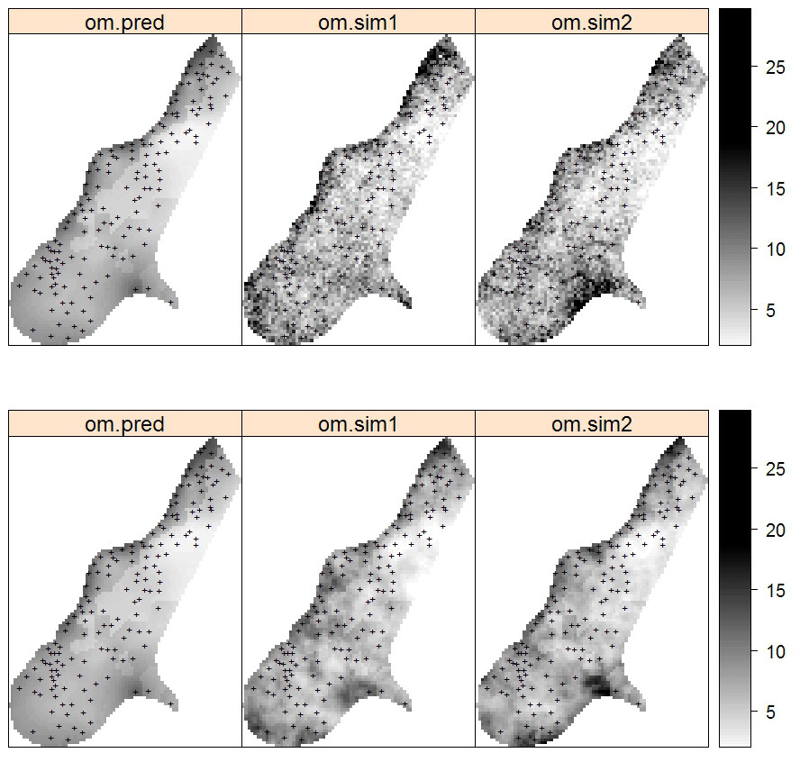
Figure 5.11: Predictions and simulations (2) at point (above) and block (below) support using the Meuse dataset. Note that prediction values produced by point and block methods are quite similar. Simulations on block support produce smoother maps than the point-support simulations.
which shows that the mapping accuracy at point support is ca. 53% of the original variance (see further Eq.(5.31)).
Note also that, cross-validation using block support in many cases is not possible because the input data needed for cross-validation are only available at point support. This basically means that, for the Meuse example, to estimate the mapping accuracy at block support we would have to revisit the study area and collect additional (composite) samples on block support that match the support size of block predictions.
Although prediction at block support is attractive because it leads to more precise predictions, the amount of variation explained by predictions at block versus point support might not differ all that much or even at all. Likewise users might not be interested in block averages and may require point predictions. Geostatistical simulations on block support can also be computationally intensive and extra field effort is almost certain to be necessary to validate these maps.
One can use point samples to produce both point and block predictions, but it is more difficult to produce point predictions from block observations. This can be done using area-to-point kriging (Kyriakidis 2004), but this technique is computationally intensive, yields large prediction uncertainties, and is hampered by the fact that it requires the point support variogram which cannot uniquely be derived from only block observations.
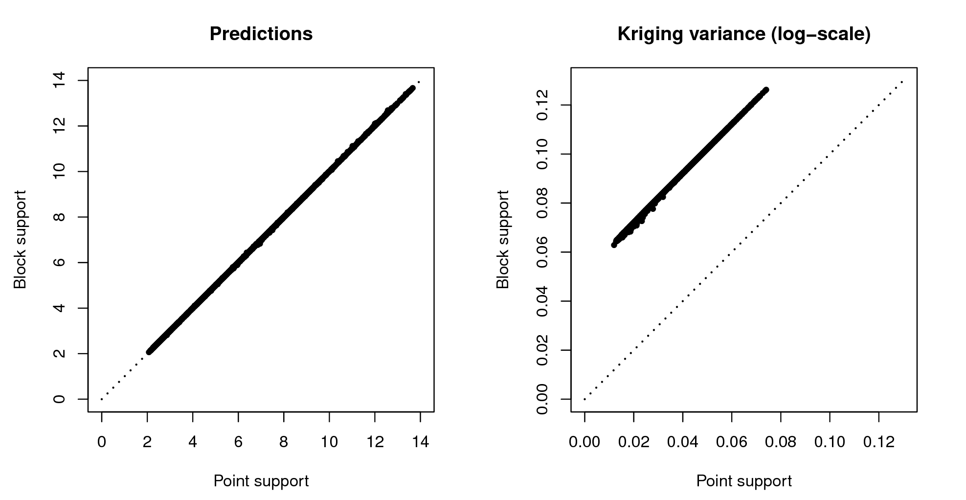
Figure 5.12: Correlation plots for predictions and prediction variance: point vs block support.
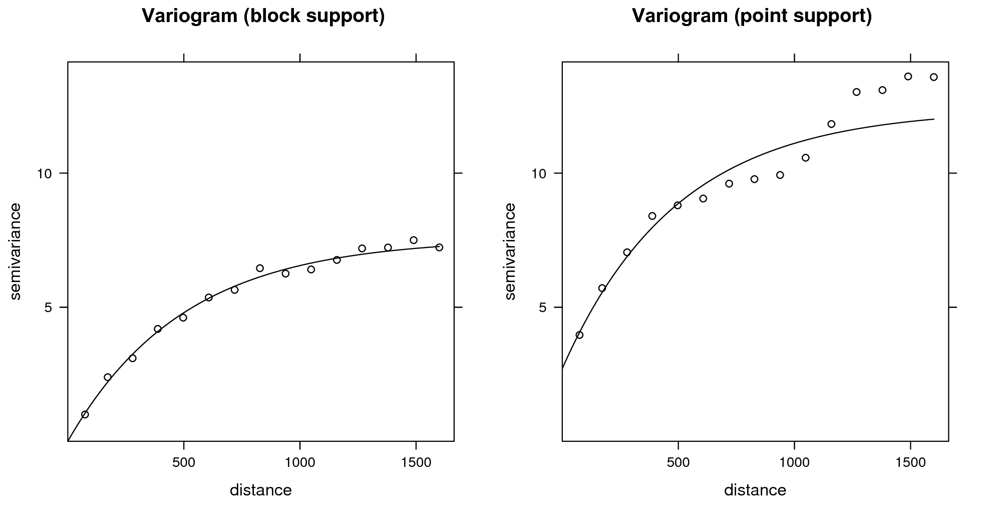
Figure 5.13: Difference in variograms sampled from the simulated maps: point vs block support.
What confuses non-geostatisticians is that both point and block predictions are normally visualized using raster GIS models, hence one does not see that the point predictions refer to the centres of the grid cells (Hengl 2006). In the case of soil survey, the available soil profile data most typically refer to point locations (\(1\times 1\) meter or smaller horizontal blocks) because soil samples have small support. In some cases surveyors mix soil samples from several different profle locations to produce composite estimates of values. Nevertheless, we can assume that the vast majority of soil profiles that are collected in the world refer to (lateral) point support. Hence the most typical combination of support size that we work with is: point support for soil property observations, block support for covariates and point or block support for soil property predictions. Modelling at full point support (both soil samples, covariates and outputs at point support) is in fact very rare. Soil covariates are often derived from remote sensing data, which is almost always delivered at block support.
In principle, there is no problem with using covariates at block support to predict the soil at point support, except the strength of the relationship between the covariate and target soil property may be weakened by a mismatch in the support. Ideally, one should always try to collect all input data at the finest support possible, then aggregate based on the project requirements. This is unfortunately not always possible, as most inputs are often bulked already and our knowledge about the short range variation is often very limited.
Figs. 5.12 and 5.13 (correlation plots for Meuse data set) confirms that: (1) predictions on block and point support show practically no differences and (2) the difference in the prediction error variance for point and block kriging effectively equals the nugget variance.
The targeted support size for the GlobalSoilMap project, for example, is 3–arcsecond (ca. 100 m) horizontal dimensions of the SRTM and other covariate data layers used to support prediction of spatial variation in soil properties. This project probably needs predictions at both point and block support at the target resolution, and then also provide aggregated values at coarser resolution blocks (250, 500, 1000 m etc). In any case, understanding consequences of aggregating spatial data and converting from point to block support is important.
5.2.12 Geostatistical simulations
In statistical terms, the assessment of the uncertainty of produced maps is equally important as the prediction of values at all locations. As shown in the previous section, uncertainty of soil variables can be assessed in several ways. Three aspects, however, appear to be important for any type of spatial prediction model:
What are the conditional probability distribution functions (PDFs) of the target variable at each location?
Where does the prediction model exhibit its largest errors?
What is the accuracy of the spatial predictions for the entire area of interest? And how accurate is the map overall?
For situations in which PDFs can be estimated ‘reliably’, Heuvelink and Brown (2006) argued that they confer a number of advantages over non-probabilistic techniques. For example, PDFs include methods for describing interdependence or correlation between uncertainties, methods for propagating uncertainties through environmental models and methods for tracing the sources of uncertainty in environmental data and models (Heuvelink 1998). By taking a geostatistical approach, kriging not only yields prediction maps, but also automatically produces PDFs at prediction points and quantifies the spatial correlation in the prediction errors. Geostatistical simulation, as already introduced in previous sections, refers to a method where realizations are drawn from the conditional PDF using a pseudo-random number generator. These simulations give a more realistic image of the spatial correlation structure or spatial pattern of the target variable because, unlike kriging, they do not smooth out the values.
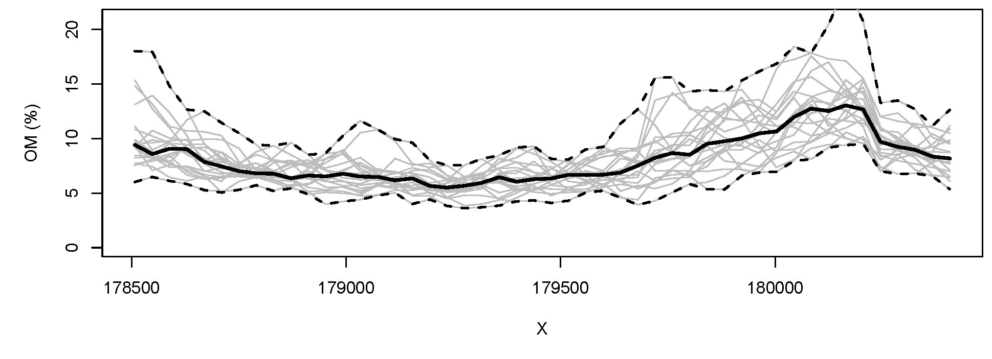
Figure 5.14: 20 simulations (at block support) of the soil organic carbon for the Meuse study area (cross-section from West to East at Y=330348). Bold line indicates the median value and broken lines indicate upper and lower quantiles (95% probability).
Estimates of the model accuracy are also provided by the geostatistical model, i.e. the kriging variance. It is useful to note that the variance of a large number of geostatistical simulations will approximate the kriging variance (and likewise the average of a large number of simulations will approximate the kriging prediction map).
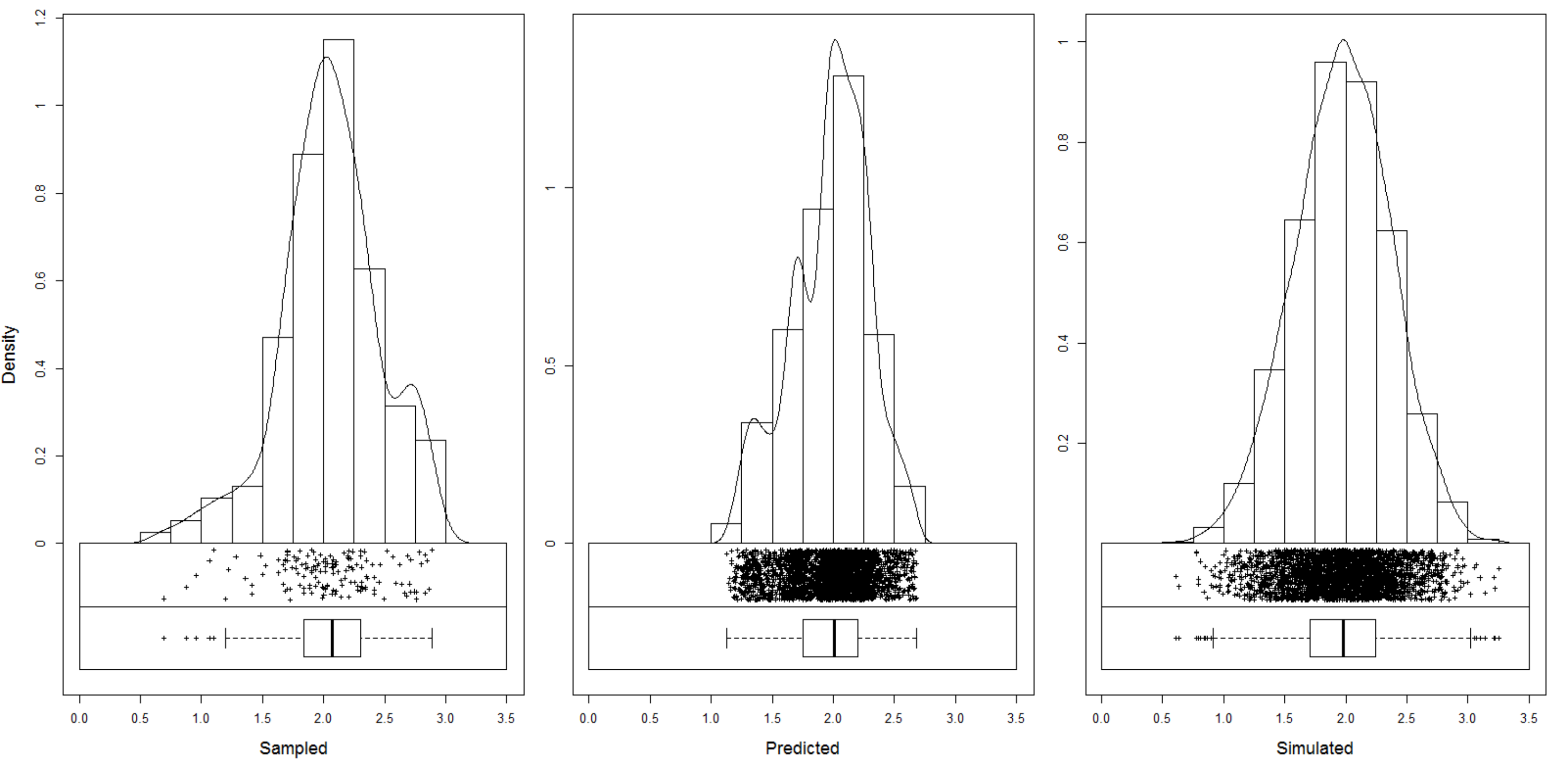
Figure 5.15: Histogram for the target variable (Meuse data set; log of organic matter) based on the actual observations (left), predictions at all grid nodes (middle) and simulations (right). Note that the histogram for predicted values will always show somewhat narrower distribution (smoothed), depending on the strength of the model, while the simulations should be able to reproduce the original range (for more discussion see also: Yamamoto et al. (2008)).
The differences among an ensemble of realizations produced using geostatistical simulations capture the uncertainty associated with the prediction map and can be used to communicate uncertainty or used as input in a spatial uncertainty propagation analysis.
Even though the kriging variance and geostatistical simulations are valid and valuable means to quantify the prediction accuracy, it is important to be aware that these assessments of uncertainty are model-based, i.e. are only valid under the assumptions made by the geostatistical model. A truly model-free assessment of the map accuracy can (only) be obtained by probability-based validation (Brus, Kempen, and Heuvelink 2011). For this we need an independent sample i.e. a sample that was not used to build the model and make the predictions, and that, in addition, was selected from the study area using a probabilistic sampling design.
For the regression-kriging model fitted for organic carbon of the Meuse
data set, we can produce 20 simulations by switching the nsim
argument:
om.rksim.p <- predict(omm, meuse.grid, block=c(0,0), nsim=20)
#> Subsetting observations to fit the prediction domain in 2D...
#> Generating 20 conditional simulations using the trend model (RK method)...
#> drawing 20 GLS realisations of beta...
#> [using conditional Gaussian simulation]
#>
100% done
#> Creating an object of class "RasterBrickSimulations"
log1p(meuse@data[1,"om"])
#> [1] 2.7
extract(raster(om.rk.p@predicted), meuse[1,])
#> [1] 2.7
extract(om.rksim.p@realizations, meuse[1,])
#>      sim1 sim2 sim3 sim4 sim5 sim6 sim7 sim8 sim9 sim10 sim11 sim12 sim13
#> [1,]  2.3  2.8  2.8  2.9  2.2  2.4  2.8  2.4  2.4     2   2.3   2.9   2.8
#>      sim14 sim15 sim16 sim17 sim18 sim19 sim20
#> [1,]   2.7   2.5   2.9   2.7   2.8   2.4   2.5
which shows the difference between sampled value (2.681022), predicted value (2.677931) and simulated values for about the same location i.e. a PDF (see also histograms in Fig. 5.15). If we average the 20 simulations we obtain an alternative estimate of the mean:
mean(extract(om.rksim.p@realizations, meuse[1,]))
#> [1] 2.6
In this case there remains a small difference between the two results, which is probably due to the small number of simulations (20) used.
5.2.13 Automated mapping
Applications of geostatistics today suggest that we will be increasingly
using automated mapping algorithms for mapping environmental
variables. The authors of the intamap package for R, for example, have
produced a wrapper function interpolate that automatically generates
predictions for any given combiination of input observations and prediction locations
(Pebesma et al. 2011). Consider the following example for predicting
organic matter content using the Meuse case study:
library(intamap)
#>
#> Attaching package: 'intamap'
#> The following object is masked from 'package:raster':
#>
#>     interpolate
demo(meuse, echo=FALSE)
meuse$value = meuse$zinc
output <- interpolate(meuse, meuse.grid, list(mean=TRUE, variance=TRUE))
#> R 2019-03-17 17:05:16 interpolating 155 observations, 3103 prediction locations
#> Warning in predictTime(nObs = dim(observations)[1], nPred = nPred, formulaString = formulaString, :
#>  using standard model for estimating time. For better
#>  platform spesific predictions, please run
#>  timeModels <- generateTimeModels()
#>   and save the workspace
#> [1] "estimated time for  copula 155.265554328003"
#> Checking object ... OK
which gives the (presumably) best interpolation method for the problem
at hand (value column), given the time available set with
maximumTime (Pebesma et al. 2011):
str(output, max.level = 2)
#> List of 16
#>  $ observations       :Formal class 'SpatialPointsDataFrame' [package "sp"] with 5 slots
#>  $ formulaString      :Class 'formula'  language value ~ 1
#>   .. ..- attr(*, ".Environment")=<environment: 0x14e195e8>
#>  $ predictionLocations:Formal class 'SpatialPixelsDataFrame' [package "sp"] with 7 slots
#>  $ params             :List of 18
#>   ..$ doAnisotropy     : logi TRUE
#>   ..$ testMean         : logi FALSE
#>   ..$ removeBias       : logi NA
#>   ..$ addBias          : logi NA
#>   ..$ biasRemovalMethod: chr "LM"
#>   ..$ nmax             : num 50
#>   ..$ nmin             : num 0
#>   ..$ omax             : num 0
#>   ..$ maxdist          : num Inf
#>   ..$ ngrid            : num 100
#>   ..$ nsim             : num 100
#>   ..$ sMin             : num 4
#>   ..$ block            : num(0)
#>   ..$ processType      : chr "gaussian"
#>   ..$ confProj         : logi TRUE
#>   ..$ debug.level      : num 0
#>   ..$ nclus            : num 1
#>   ..$ significant      : logi TRUE
#>   ..- attr(*, "class")= chr "IntamapParams"
#>  $ outputWhat         :List of 2
#>   ..$ mean    : logi TRUE
#>   ..$ variance: logi TRUE
#>  $ blockWhat          : chr "none"
#>  $ intCRS             : chr "+init=epsg:28992 +proj=sterea +lat_0=52.15616055555555 +lon_0=5.38763888888889 +k=0.9999079 +x_0=155000 +y_0=46"| __truncated__
#>  $ lambda             : num -0.27
#>  $ anisPar            :List of 4
#>   ..$ ratio     : num 1.48
#>   ..$ direction : num 56.1
#>   ..$ Q         : num [1, 1:3] 3.05e-07 2.29e-07 -9.28e-08
#>   .. ..- attr(*, "dimnames")=List of 2
#>   ..$ doRotation: logi TRUE
#>  $ variogramModel     :Classes 'variogramModel' and 'data.frame':    2 obs. of  9 variables:
#>   ..$ model: Factor w/ 20 levels "Nug","Exp","Sph",..: 1 3
#>   ..$ psill: num [1:2] 0.00141 0.02527
#>   ..$ range: num [1:2] 0 1282
#>   ..$ kappa: num [1:2] 0 0
#>   ..$ ang1 : num [1:2] 0 33.9
#>   ..$ ang2 : num [1:2] 0 0
#>   ..$ ang3 : num [1:2] 0 0
#>   ..$ anis1: num [1:2] 1 0.674
#>   ..$ anis2: num [1:2] 1 1
#>   ..- attr(*, "singular")= logi FALSE
#>   ..- attr(*, "SSErr")= num 2.84e-08
#>   ..- attr(*, "call")= language fit.variogram(object = experimental_variogram, model = vgm(psill = psill,      model = model, range = range, nugg| __truncated__ ...
#>  $ sampleVariogram    :Classes 'gstatVariogram' and 'data.frame':    11 obs. of  6 variables:
#>   ..$ np     : num [1:11] 7 31 94 132 147 ...
#>   ..$ dist   : num [1:11] 67.2 94.2 142.9 193.5 248.9 ...
#>   ..$ gamma  : num [1:11] 0.000891 0.005635 0.005537 0.006056 0.010289 ...
#>   ..$ dir.hor: num [1:11] 0 0 0 0 0 0 0 0 0 0 ...
#>   ..$ dir.ver: num [1:11] 0 0 0 0 0 0 0 0 0 0 ...
#>   ..$ id     : Factor w/ 1 level "var1": 1 1 1 1 1 1 1 1 1 1 ...
#>   ..- attr(*, "direct")='data.frame':    1 obs. of  2 variables:
#>   ..- attr(*, "boundaries")= num [1:12] 36.8 73.5 110.3 165.5 220.6 ...
#>   ..- attr(*, "pseudo")= num 0
#>   ..- attr(*, "what")= chr "semivariance"
#>  $ methodParameters   : chr "  vmodel = data.frame(matrix(0,nrow =  2 ,ncol =  9 ))\nnames(vmodel) = c(\"model\",\"psill\",\"range\",\"kappa"| __truncated__
#>  $ predictions        :Formal class 'SpatialPixelsDataFrame' [package "sp"] with 7 slots
#>  $ outputTable        : num [1:4, 1:3103] 181180 333740 842 44785 181140 ...
#>   ..- attr(*, "dimnames")=List of 2
#>   ..- attr(*, "transposed")= logi TRUE
#>  $ processPlot        : chr ""
#>  $ processDescription : chr "Spatial prediction using the method  transGaussian"
#>  - attr(*, "class")= chr "transGaussian"
The interpolate function automatically chooses between: (1) kriging, (2) copula methods, (3) inverse distance interpolation, projected spatial gaussian process methods in the gstat package, (4) transGaussian kriging or Yamamoto interpolation.
The same idea of automated model fitting and prediction has been implemented in the GSIF package. Some examples of automated soil mapping have been already shown previously.
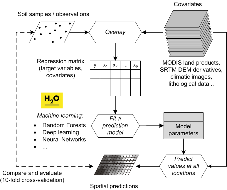
Figure 5.16: A modern workflow of predictive soil mapping. This often includes state-of-the-art Machine Learning Algorithms. Image source: Hengl et al. (2017) doi: 10.1371/journal.pone.0169748.
Automated mapping, as long as it is not a black-box system, is beneficial for soil mapping applications for several reasons: (1) it saves time and effort needed to get initial results, (2) it allows generation of maps using current data (live geostatistics) even via a web-interfaces, (3) it greatly reduces the workload in cases where maps need to be produced repeatedly, such as when regular updates are needed or the same model is applied in different subareas. In practice, automated mapping is typically a three-stage process (Fig. 5.16):
Rapidly generate predictions and a report of analysis (analyze why a particular technique was chosen and how well it performs? Are there any outliers or artifacts? Which predictors are most significant? etc).
Review the results of spatial prediction and fine-tune some parameters and if necessary filter and/or adjust the input maps.
Re-run the prediction process and publish the final maps.
hence geostatisticians are still an essential and active part of the process. In automated mapping they primarily focus their expertise on doing interpretation of the results rather than on manually analyzing the data.
It is unlikely that a simple linear prediction model can be used to fit every type of soil data. It is more likely that some customized models, i.e. models specific for each property, would perform better than if a single model were used for a diversity of soil properties. This is because different soil properties have different distributions, they vary differently at different scales, and are controlled by different processes. On the other hand, the preferred way to ensure that a single model can be used to map a variety of soil properties is to develop a generic framework with multi-thematic, multi-scale predictors that allows for iterative search for optimal model structure and parameters, and then implement this model via an automated mapping system.
5.2.14 Selecting spatial prediction models
The purpose of spatial prediction is to (a) produce a map showing spatial distribution of the variable of interest for the area of interest, and (b) to do this in an unbiased way. A comprehensive path to evaluating spatial predictions is the caret approach (Kuhn and Johnson 2013), which wraps up many of the standard processes such as model training and validation, method comparison and visualization. Consider, for example, organic matter % in the topsoil in the meuse data set:
library(caret); library(rgdal)
#> Loading required package: lattice
#> Loading required package: ggplot2
#>
#> Attaching package: 'caret'
#> The following object is masked from 'package:intamap':
#>
#>     preProcess
demo(meuse, echo=FALSE)
meuse.ov <- cbind(over(meuse, meuse.grid), meuse@data)
meuse.ov$x0 = 1
We can quickly compare performance of using GLM vs random forest vs no model for predicting organic matter (om) by using the caret package functionality:
fitControl <- trainControl(method="repeatedcv", number=2, repeats=2)
mFit0 <- caret::train(om~x0, data=meuse.ov, method="glm",
               family=gaussian(link=log), trControl=fitControl,
               na.action=na.omit)
mFit1 <- caret::train(om~soil, data=meuse.ov, method="glm",
               family=gaussian(link=log), trControl=fitControl,
               na.action=na.omit)
mFit2 <- caret::train(om~dist+soil+ffreq, data=meuse.ov, method="glm",
               family=gaussian(link=log), trControl=fitControl,
               na.action=na.omit)
mFit3 <- caret::train(om~dist+soil+ffreq, data=meuse.ov, method="ranger",
               trControl=fitControl, na.action=na.omit)
This will run repeated Cross-validation with 50% : 50% splits training and validation, which means that, in each iteration, models will be refitted from scratch. Next we can compare performance of the three models by using:
resamps <- resamples(list(Mean=mFit0, Soilmap=mFit1, GLM=mFit2, RF=mFit3))
bwplot(resamps, layout = c(2, 1), metric=c("RMSE","Rsquared"),
       fill="grey", scales = list(relation = "free", cex = .7),
       cex.main = .7, cex.axis = .7)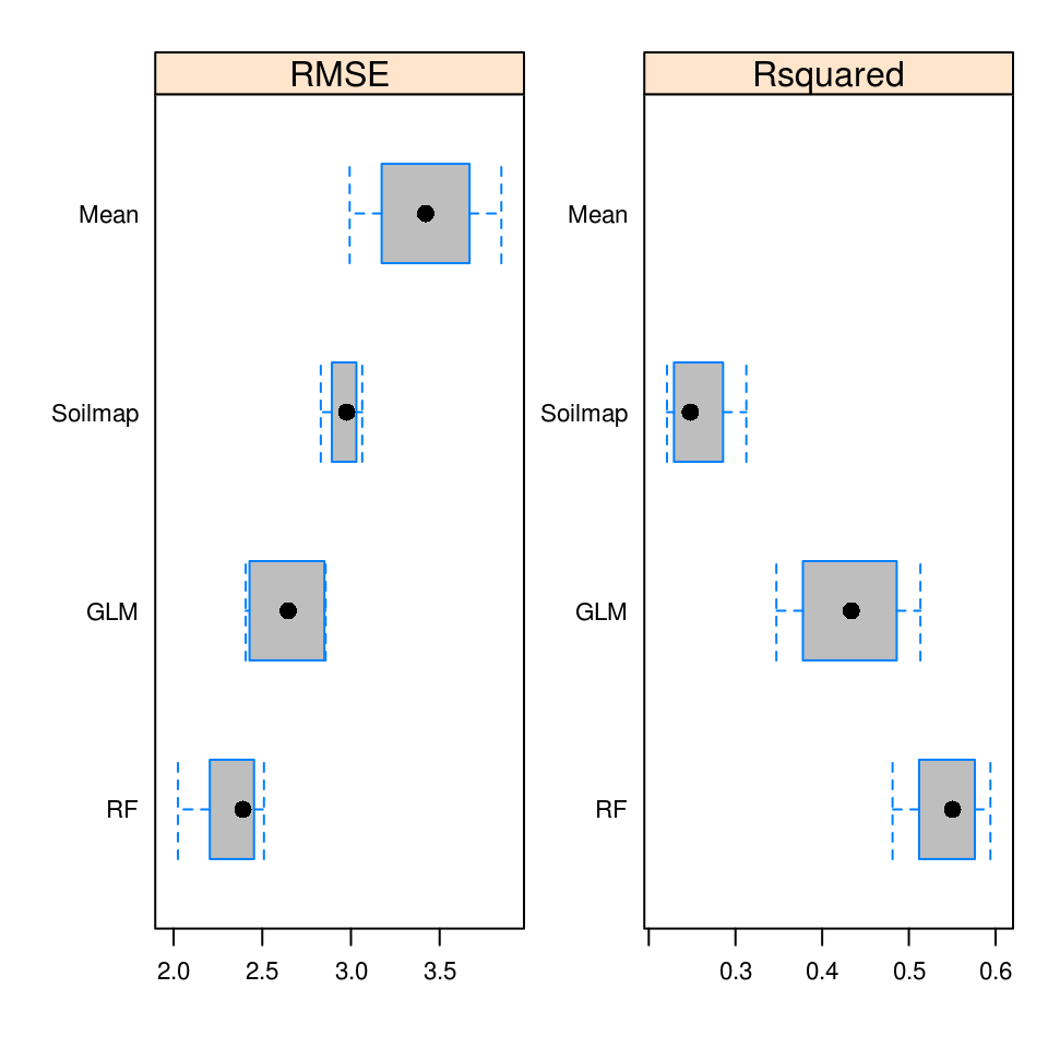
Figure 5.17: Comparison of spatial prediction accuracy (RMSE at cross-validation points) for simple averaging (Mean), GLM with only soil map as covariate (Soilmap), GLM and random forest (RF) models with all possible covariates. Error bars indicate range of RMSE values for repeated CV.
In the case above, it seems that random forest (ranger package) helps reduce mean RMSE of predicting organic matter by about 32%:
round((1-min(mFit3$results$RMSE)/min(mFit0$results$RMSE))*100)
#> [1] 32
There is certainly added value in using spatial covariates (in the case above: distance to water and flooding frequency maps) and in using machine learning for spatial prediction, even with smaller data sets.
Note also that the assessment of spatial prediction accuracy for the three models based on the train function above is model-free, i.e. cross-validation of the models is independent of the models used because, at each cross-validation subset, fitting of the model is repeated and validation points are maintained separate from model training. Subsetting point samples is not always trivial however: in order to consider cross-validation as completely reliable, the samples ought to be representative of the study area and preferably collected using objective sampling such as simple random sampling or similar (Brus, Kempen, and Heuvelink 2011; Brus 2019). In cases where the sampling locations are clustered in geographical space i.e. if some parts of the study area are completely omitted from sampling, then also the results of cross-validation will reflect that sampling bias / poor representation. In all the following examples we will assume that cross-validation gives a reliable measure of mapping accuracy and we will use it as the basis of accuracy assessment i.e. mapping efficiency. In reality, cross-validation might be tricky to implement and could often lead to somewhat over-optimistic results if either sampling bias exists or/and if there are too few points for model validation. For example, in the case of soil profile data, it is highly recommended that entire profiles are removed from CV because soil horizons are too strongly correlated (as discussed in detail in Gasch et al. (2015) and Brenning (2012)).
The whole process of spatial prediction of soil properties could be summarized in 5 steps:
- Initial model comparison (comparison of prediction accuracy and computing time).
- Selection of applicable model(s) and estimation of model parameters i.e. model fitting.
- Predictions i.e. generation of maps for all areas of interest.
- Objective accuracy assessment using independent (cross-)validation.
- Export and sharing of maps and summary documentation explaining all processing steps.
Studying the caret package tutorial and/or the mlr tutorials is highly recommended for anyone looking for a systematic introduction to predictive modelling.
5.2.15 3D regression-kriging
Measurements of soil properties at point support can be thought of as describing explicit 3D locations (easting, northing and depth), and are amenable to being dealt with using 3D geostatistics (e.g. 3D kriging). Application of 3D kriging to soil measurements is cumbersome for several reasons:
The differences between sampling intervals and spatial correlation in the horizontal and vertical dimensions are very large (<10 in the vertical v.s. 100’s to 1000’s of in the horizontal). The resulting strong anisotropy must be accounted for when the geostatisitcal model is derived. Estimation of the anisotropy may be hampered by the relatively small number of observations along the vertical profile, although under a stationarity assumption it can benefit from the many repetitions of profile data for all profile locations.
Soil property values refer to vertical block support (usually because they are composite samples, i.e. the average over a soil horizon), hence some of the local variation (in the vertical dimension) has been smoothed out.
Soil surveyors systematically under-represent lower depths — surveyors tend to systematically take fewer samples as they assume that deeper horizons are of less importance for management or because deeper horizons are more expensive to collect or because deeper horizons are assumed to be more homogeneous and uniform.
Many soil properties show clear trends in the vertical dimension and, if this is ignored, the result can be a very poor geostatistical model. It may not be that easy to incorporate a vertical trend because such a trend is generally not consistently similar between different soil types. On the other hand, soil variables are auto-correlated in both horizontal and vertical (depth) dimensions, so that it makes sense to treat them using 3D geostatistics whenever we have enough 3D soil observations.
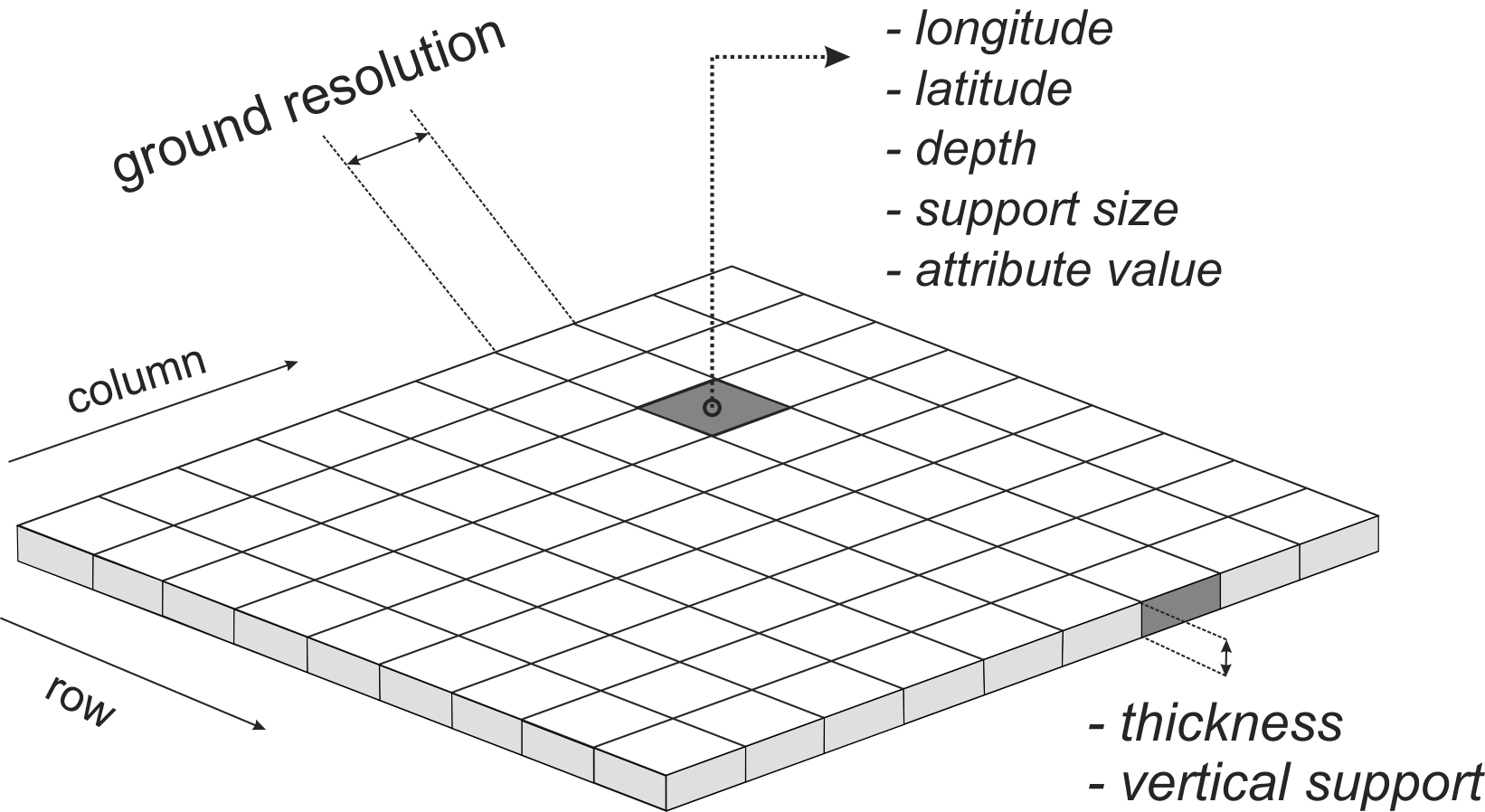
Figure 5.18: Spatial 3D prediction locations in a gridded system (voxels). In soil mapping, we often predict for larger blocks of land e.g. 100 to 1000 m, but then for vertical depths of few tens of centimeters, so the output voxels might appear in reality as being somewhat disproportional.
The fact that there are almost always <10 soil observations over the total depth of a soil profile, so that the estimates of the range in the vertical dimension will be relatively poor, is something that cannot be improved. The fact that soil samples taken by horizon refer to block support is a more serious problem, as part of short range variation has been lost, plus we know that the point values do not refer to the horizon center but to the whole horizon block, which, in addition to everything else, tend to be irregular i.e. do not have constant depth and width.
To predict in 3D space, we extend the regression model from Eq.(5.10) with a soil depth function:
\[\begin{equation} \begin{split} \hat z({{s}}_0, d_0 ) = \sum\limits_{j = 0}^p {\hat \beta _j \cdot X_j ({{s}}_0, d_0 )} + {{\hat g}}(d_0) + \sum\limits_{i = 1}^n {\hat{\lambda}_i ({{s}}_0, d_0 ) \cdot e({{s}}_i, d_i )} \end{split} \tag{5.25} \end{equation}\]where \(d\) is the 3rd depth dimension expressed in meters from the land surface, \({{\hat g}}(d_0)\) is the predicted soil depth function, typically modelled by a spline function. This allows prediction of soil properties at any depth using observations at other depths but does require 3D modelling of the covariance structure, which is not easy because there may be zonal and geometric anisotropies (i.e. the variance and correlation lengths may differ between vertical and horizontal directions). Also, the vertical support of observations becomes important and it should be realized that observations are the averages over depth intervals and not values at points along the vertical axis (Fig. 5.18). Spline functions have been proposed and used as mass-preserving curve fitting methods to derive point and block values along the vertical axis from observations at given depth intervals, but the difficulty is that these yield estimates (with uncertainties) that should not be confused with real observations.
A 3D variogram, e.g. modelled using an exponential model with three standard parameters (nugget \(c_0\), partial sill \(c_1\), range parameter \(r\)):
\[\begin{equation} \gamma \left( {{h}} \right) = \left\{ {\begin{array}{*{20}c} 0 & {{\rm{if}}} & {h = 0} \\ {c_0 + c_1 \cdot \left[ {1 - e^{ - \left( {\frac{{h}} {r}} \right)} } \right]} & {{\rm{if}}} & {h > 0} \\ \end{array} } \right. \qquad {{h}} = \left[ {h_x , h_y , h_d } \right] \tag{5.26} \end{equation}\]where the scalar ‘distance’ \(h\) is calculated by scaling horizontal and vertical separation distances using three anisotropy parameters:
\[\begin{equation} h = \sqrt {\left( {\frac{{h_x }}{{a_x }}} \right)^2 + \left( {\frac{{h_y }}{{a_y }}} \right)^2 + \left( {\frac{{h_d }}{{a_d }}} \right)^2 } \tag{5.27} \end{equation}\]Typically, in the case of soil data, the anisotropy ratio between horizontal and vertical distances is high — spatial variation observed in a few depth changes may correspond with several or more in horizontal space, so that the initial settings of the anisotropy ratio (i.e. the ratio of the horizontal and vertical variogram ranges) are between 3000–8000, for example. Variogram fitting criteria can then be used to optimize the anisotropy parameters. In our case we assumed no horizontal anisotropy and hence assumed \(a_x=a_y=1\), leaving only \(a_d\) to be estimated. Once the anisotropy ratio is obtained, 3D variogram modelling does not meaningfully differ from 2D variogram modelling.
The 3D RK framework explained above can be compared to the approach of Malone et al. (2009), who first fit an equal-area spline function to estimate the soil properties at standard depths, and next fit regression and variogram models at each depth. A drawback of the approach by Malone et al. (2009), however, is that the separate models for each depth ignore all vertical correlations. In addition, the equal-area spline is not used to model soil-depth relationships but only to estimate the values at standard depths for sampling locations i.e. it is implemented for each soil profile (site) separately. In the 3D RK framework explained above, a single model is used to generate predictions at any location and for any depth, and this takes into account both horizontal and vertical relationships simultaneously. The 3D RK approach is both easier to implement, and allows for incorporating all (vertical) soil-depth relationships including the spatial correlations.
5.2.16 Predicting with multiscale and multisource data
Fig. 5.3 indicates that spatial prediction is a
linear processes with one line of inputs and one line of outputs. In
some cases soil mappers have to use methods that can work with
multi-scale and/or multi-source data i.e. data with different
extents, resolution and uncertainty. Here by multiscale data we imply
covariates used for geostatistical mapping that are available at two or
more (distinctly different) resolutions, but that cover the same area of
interest (see also: RasterStack class in the raster package). In the case of
the multisource data, covariates can be of any scale, they can have a
variable extent, and variable accuracy
(Fig. 5.19b). In other words, when
referring to multiscale data, we assume that the input covariate layers
differ only in their resolution; whereas in referring to multisource data, we
consider that all technical aspects of the input data could potentially be
different.
Organizing (and using) multiscale and multisource data is something that probably can not be avoided in global soil mapping projects. From the GIS perspective, and assuming a democratic right to independently develop and apply spatial prediction models, merging of the multiscale and multisource data is likely to be inevitable.
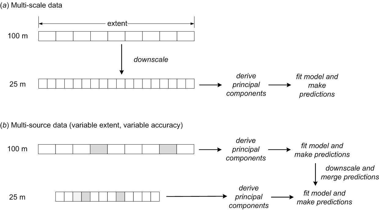
Figure 5.19: A general scheme for generating spatial predictions using multiscale and multisource data.
As a general strategy, for multi-scale data, a statistically robust approach is to fit a single model to combined covariates downscaled or upscaled to a single, common resolution (Fig. 5.19a). For the multi-source data data assimilation methods i.e. merging of predictions (Fig. 5.19b) can be used (Caubet et al. 2019). Imagine if we have covariate layers for one whole continent at some coarse resolution of e.g. 500 m, but for some specific country have other predictions at a finer resolution of e.g. 100 m. Obviously any model we develop that uses both sources of data is limited in its application to just the extent of that country. To ensure that all covariate and soil data available for that country are used to generate predictions, we can fit two models at seperate scales and independently of each other, and then merge the predictions only for the extent of the country of interest. A statistical framework for merging such predictions is given, for example, in Caubet et al. (2019). In that sense, methods for multisource data merging are more attractive for pan-continental and global projects, because for most of the countries in the world, both soil and covariate data are available at different effective scales.
It is important to emphasize, however, that, in order to combine various predictors, we do need to have an estimate of the prediction uncertainty e.g. derived using cross-validation, otherwise we are not able to assign the weights. In principle, a linear combination of statistical techniques using the equation above should be avoided if a theoretical basis exists that incorporates such a combination.
Combined predictions are especially interesting for situations where:
predictions are produced using different inputs i.e. data with different coverage,
there are several prediction methods which are equally applicable,
where no theory exists that describes a combination of spatial prediction methods,
where fitting and prediction of individual models is faster and less problematic than fitting of a hybrid model.
Estimation of the prediction variance and confidence interval of combined or merged predictions is more complex than estimation of the mean value.
5.3 Accuracy assessment and the mapping efficiency
5.3.1 Mapping accuracy and numeric resolution
Every time a digital soil mapper produces soil maps, soil GIS and soil geographical databases those products can be evaluated using independent validation studies. Unfortunately, much evaluation of soil maps in the world is still done using subjective ‘look-good’ assessments and the inherent uncertainty of the product is often underreported. In this book, we promote objective assessment of mapping accuracy, i.e. based on statistical testing using ground truth data.
Mapping accuracy can be defined as the difference between an estimated value and the “true” value, i.e. a value of the same target variable arrived at using a significantly more accurate method. In the most simple terms, accuracy is the error component of the perfectly accurate map (Mowrer and Congalton 2000). Although we know that soils form under systematic environmental conditions and probably much of the variation is deterministic (Eq.(5.1)), we do not yet have tools that allow us to model soil formation and evolution processes perfectly (see also section 1.6.2). The best we can do is to calibrate some spatial prediction model using field records, and then generate (the best possible) predictions. The resulting soil property map, i.e. what we know about soils, is then a sum of two signals:
\[\begin{equation} z^{\rm{map}}({{s}}) = Z({{s}}) + \varepsilon({{s}}) \tag{5.28} \end{equation}\]where \(Z({{s}})\) is the true variation, and \(\varepsilon({{s}})\) is the error component i.e. what we do not know. The error component, also known as the error budget, consists of two parts: (1) the unexplained part of soil variation, and (2) the pure noise (sampling and measurement errors described in section 1.6.2).
The unexplained part of soil variation is the variation we somehow failed to explain because we are not using all relevant covariates and/or due to the limited sampling intensity. For example, the sampling plan might fail to sample some hot-spots or other important local features. The unexplained part of variation also includes short-range variation, which is possibly deterministic but often not of interest or is simply not feasible to describe at common mapping scales.
The way to determine the error part in Eq.(5.28) is to collect additional samples and then determine the average error or the Root Mean Square Error (Goovaerts 2001; Finke 2006; Li and Heap 2010):
\[\begin{equation} {\it RMSE} = \sqrt {\frac{1}{l} \cdot \sum\limits_{i = 1}^l {\left[ {\hat z({{s}}_i ) - z ({{s}}_i )} \right]^2 } } \tag{5.29} \end{equation}\]where \(l\) is the number of validation points, and the expected estimate of prediction error at sampling locations is equal to the nugget variation (\(E\{ {\it RMSE} \} = \sigma({{h}}=0)\)). In addition to \(\it{RMSE}\), it is often interesting to see also whether the errors are, on average, positive (over-estimation) or negative (under-estimation) i.e. whether there is possibly any clear bias in our predictions:
\[\begin{equation} {\rm ME} = \frac{1}{m} \sum_{j=1}^{m} (\hat y ({ s}_j) - y ({ s}_j)) \tag{5.30} \end{equation}\]To see how much of the global variation budget has been explained by the model we can use:
\[\begin{equation} {\Sigma}_{\%} = \left[ 1 - \frac{{\it{SSE}}}{{\it{SSTO}}} \right] = \left[ 1 - \frac{{\it{RMSE}}^2}{\sigma_z^2} \right] [0-100\%] \tag{5.31} \end{equation}\]where \(\it{SSE}\) is the sum of squares for residuals at cross-validation points (i.e. \({\it{MSE}} \cdot n\)), and \(\it{SSTO}\) is the total sum of squares. \({\Sigma}_{\%}\) is a global estimate of the map accuracy, valid only under the assumption that the validation points are spatially independent from the calibration points, representative and large enough (e.g. \(l>50\)), and that the error component is normally distributed around the zero value (\(E\left\{ {\hat z({{{s}}_i}) - z({{{s}}_i})} \right\} = 0\)).
Once we have estimated \(\it{RMSE}\), we can also determine the effective numeric resolution for the predictions (Hengl, Nikolić, and MacMillan 2013). For example, assuming that the original sampling variance is 1.85 and that \(\it{RMSE}\)=1 (i.e. \({\Sigma}_{\%}\)=47%), the effective numeric resolution for predictions is then 0.5 (as shown previously in Fig. 1.16). There is probably no need to code the values with a better precision than 0.5 units.
5.3.2 Accuracy assessment methods
There are three possibilities for estimating the \(\it{RMSE}\) (Fig. 5.20):
Run cross-validation using the same input data used for model fitting.
Collect new samples using a correct probability sampling design to ensure an unbiased estimate of accuracy.
Compare predicted values with more detailed maps for small study areas produced at much higher accuracy, usually also at much finer level of detail.
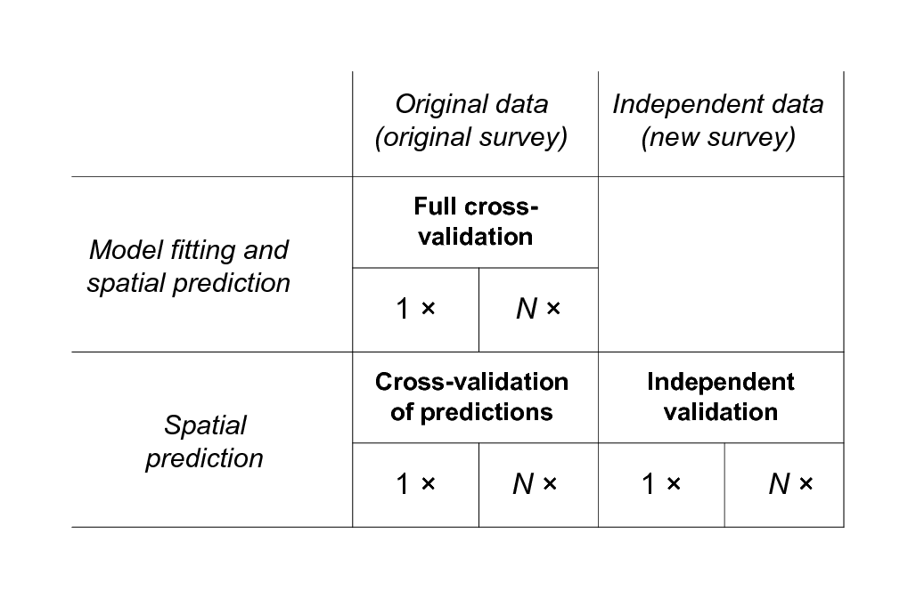
Figure 5.20: General types of validation procedures for evaluating accuracy of spatial prediction models.
Although the prediction variance already indicates what the potential accuracy of the maps is, only by independent validation can we determine the true accuracy of the maps. Brus, Kempen, and Heuvelink (2011) further show that, actually, only if the validation points are selected using some probability-based sampling, like simple random sampling or stratified sampling, can one determine the true accuracy of any produced gridded maps. In practice, we can rarely afford to collect new samples, so that cross-validation is often the only viable option.
5.3.3 Cross-validation and its limitations
Because collecting additional (independent) samples is often impractical and expensive, validation of prediction models is commonly done by using cross-validation i.e. by subsetting the original point set into two data sets — calibration and validation — and then repeating the analysis. There are several types of cross-validation methods (Bivand, Pebesma, and Rubio 2008, 221–26):
the \(k\)–fold cross-validation — the original sample is split into \(k\) equal parts and then each is used for cross-validation;
leave-one-out cross-validation (LOO) — each sampling point is used for cross-validation;
Jackknifing — similar to LOO, but aims at estimating the bias of statistical analysis and not of predictions;
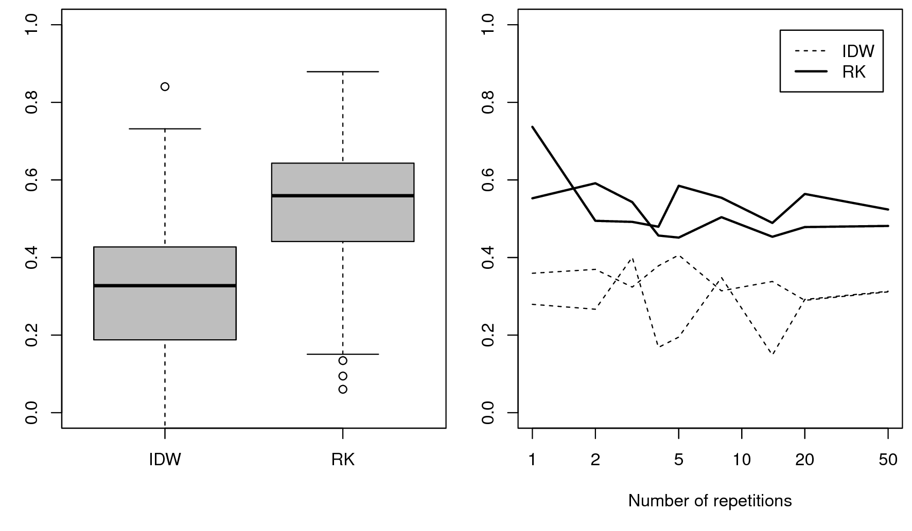
Figure 5.21: Left: confidence limits for the amount of variation explained (0–100%) for two spatial prediction methods: inverse distance interpolation (IDW) and regression-kriging (RK) for mapping organic carbon content (Meuse data set). Right: the average amount of variation explained for two realizations (5-fold cross-validation) as a function of the number of cross-validation runs (repetitions). In this case, the RK method is distinctly better than method IDW, but the cross-validation score seems to stabilize only after 10 runs.
Both \(k\)–fold and the leave-one-out cross validation are implemented in
the e.g. gstat package (krige.cv methods), which makes this type of
assessment convenient to implement. Note also that cross-validation is
not necessarily independent — points used for cross-validation are a
subset of the original sampling design, hence if the original design is
biased and/or non-representative, then also the cross-validation might
not reveal the true accuracy of a technique. However, if the sampling
design has been generated using some unbiased design based sampling
(e.g. random sampling), randomly seleced subsets will provide unbiased
estimators of the true mapping accuracy.
“Models can only be evaluated in relative terms, and their predictive value is always open to question. The primary value of models is heuristic.” (Oreskes, Shrader-Frechette, and Belitz 1994)
Hence, also in soil mapping, accuracy assessment
should only be considered in relative terms. Each evaluation of soil
mapping accuracy might give somewhat different numbers, so it is often a
good idea to repeat the evaluation multiple times. Likewise, cross-validation
requires enough repetition (e.g. at least 3) otherwise over-positive or
over-negative results can be produced by chance
(Fig. 5.21). Many geostatisticians
(see e.g. krige.cv function described in Bivand, Pebesma, and Rubio (2008, 222–23)) suggest that at least 5 repetitions are needed to produce
‘stable’ measures of the mapping accuracy. If only one realization of
cross-validation is used, this can accidentally lead to over-optimistic
or over-pessimistic estimates of the true mapping accuracy.
5.3.4 Accuracy of the predicted model uncertainty
Recall from Eq.(5.7) that the output of the prediction process is typically (1) predicted mean value at some location (\(\hat Z({{s}}_0)\)), and (2) predicted prediction variance i.e. regression-kriging error (\(\hat{\sigma}({{s}}_0)\)). In the previous section we have shown some common accuracy measures for the prediction of the mean value. It might sound confusing but, in geostatistics, one can also validate the uncertainty of uncertainty i.e. derive the error of the estimation error. In the case of the Meuse data set:
om.rk.cv <- krige.cv(log1p(om)~dist+soil, meuse.s, vr.fit)
hist(om.rk.cv$zscore, main = "Z-scores histogram",
     xlab = "z-score value", col = "grey", breaks = 25,
     cex.axis = .7, cex.main = .7, cex.lab = .7)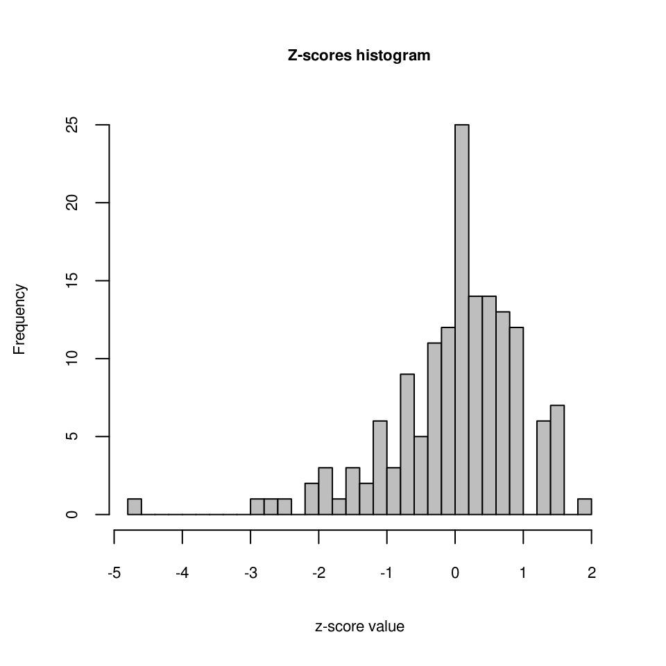
Figure 5.22: Z-scores for the cross-validation of the soil organic carbon model.
Here, the cross-validation function krige.cv reports errors at
validation points (5–fold cross-validation by default), but it also
compares the difference between the regression-kriging error estimated by
the model and the actual error. The ratio between the actual and
expected error is referred to as the \(z\)-scores (Bivand, Pebesma, and Rubio 2008, 225):
Ideally, the mean value of \(z\)-scores should be around 0 and the variance of the \(z\)-scores should be around 1. If the \(z\)-score variance is substantially smaller than \(1\), then the model overestimates the actual prediction uncertainty. If the \(z\)-score variance is substantially greater than \(1\), then the model underestimates the prediction uncertainty. The difference between the actual and predicted model error can be also referred to as the model reliability. A model can be accurate but then ‘overpessimistic’ if the predicted model uncertainty is wider than the actual uncertainty, or accurate but ‘overoptimistic’ if the reported confidence limits are too narrow (Fig. 5.23).
Ideally, we aim to produce prediction and prediction error maps that are both accurate and realistic (or at least realistic). For a review of methods for assessment of uncertainty in soil maps refer to Goovaerts (2001, 3–26) and/or Brus, Kempen, and Heuvelink (2011).
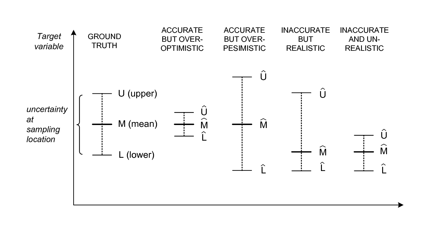
Figure 5.23: Mapping accuracy and model reliability (accuracy of the prediction intervals vs actual intervals). Although a method can be accurate in predicting the mean values, it could fail in predicting the prediction intervals i.e. the associated uncertainty.
In the case discussed above (Fig. 5.22) it appears that the error estimated by the model is often different from the actual regression-kriging variance: in this case the estimated values are often lower than actual measured values (under-estimation), so that the whole histogram shifts toward 0 value. Because the variance of the \(z\)-scores is <1:
var(om.rk.cv$zscore, na.rm=TRUE)
#> [1] 0.95
we can also say that the regression-kriging variance is slightly over-pessimistic or too conservative about the actual accuracy of the model. On the other hand, Fig. 5.22 shows that, at some points, the cross-validation errors are much higher than the error estimated by the model.
5.3.5 Derivation and interpretation of prediction interval
Another important issue for understanding the error budget is derivation of prediction interval i.e. upper and lower values of the target variable for which we assume that our predictions will fall within, with a high probability (e.g. 19 out of 20 times or the 95% probability). Prediction interval or confidence limits are commonly well accepted by users as the easiest way to communicate uncertainty (Brodlie, Osorio, and Lopes 2012). For example, organic carbon in Meuse study area (based on 153 samples of organic matter) has a 95% interval of 2–16%:
signif(quantile(meuse$om, c(.025, .975), na.rm=TRUE), 2)
#> 2.5%  98%
#>    2   16
We have previously fitted a geostatistical model using two covariates, which can now be used to generate predictions:
om.rk <- predict(omm, meuse.grid)
#> Subsetting observations to fit the prediction domain in 2D...
#> Generating predictions using the trend model (RK method)...
#> [using ordinary kriging]
#>
100% done
#> Running 5-fold cross validation using 'krige.cv'...
#> Creating an object of class "SpatialPredictions"
and which allows us to estimate the confidence limits for organic matter (assuming normal distribution) at any location within the study area e.g.:
pt1 <- data.frame(x=179390, y=330820)
coordinates(pt1) <- ~x+y
proj4string(pt1) = proj4string(meuse.grid)
pt1.om <- over(pt1, om.rk@predicted["om"])
pt1.om.sd <- over(pt1, om.rk@predicted["var1.var"])
signif(expm1(pt1.om-1.645*sqrt(pt1.om.sd)), 2)
#>    om
#> 1 4.6
signif(expm1(pt1.om+1.645*sqrt(pt1.om.sd)), 2)
#>    om
#> 1 8.9
where 4.6–8.9 are the upper and lower confidence limits. This interval can also be expressed as:
signif((expm1(pt1.om+1.645*sqrt(pt1.om.sd)) -
       expm1(pt1.om-1.645*sqrt(pt1.om.sd)))/2, 2)
#>    om
#> 1 2.1
or 6.3 ± 2.1 where half the error of estimating organic matter at that location is about 1 s.d. Note that these are location specific prediction intervals and need to be computed for each location.
To visualize the range of values within different strata, we can use simulations that we can generate using the geostatistical model (which can be time-consuming to compute!):
om.rksim <- predict(omm, meuse.grid, nsim=5, debug.level=0)
#> Subsetting observations to fit the prediction domain in 2D...
#> Generating 5 conditional simulations using the trend model (RK method)...
#> Creating an object of class "RasterBrickSimulations"
ov <- as(om.rksim@realizations, "SpatialGridDataFrame")
meuse.grid$om.sim1 <- expm1(ov@data[,1][meuse.grid@grid.index])
meuse.grid$om.rk <- expm1(om.rk@predicted$om)
par(mfrow=c(1,2))
boxplot(om~ffreq, omm@regModel$data, col="grey",
    xlab="Flooding frequency classes",
    ylab="Organic matter in %",
    main="Sampled (N = 153)", ylim=c(0,20),
    cex.axis = .7, cex.main = .7, cex.lab = .7)
boxplot(om.sim1~ffreq, meuse.grid, col="grey",
    xlab="Flooding frequency classes",
    ylab="Organic matter in %",
    main="Predicted (spatial simulations)", ylim=c(0,20),
    cex.axis = .7, cex.main = .7, cex.lab = .7)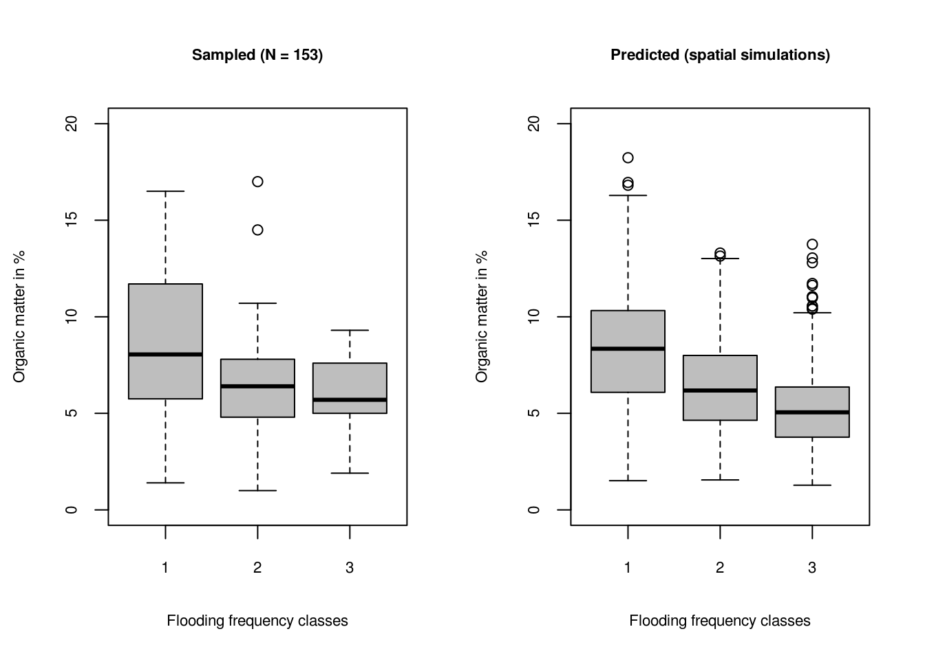
Figure 5.24: Prediction intervals for three flooding frequency classes for sampled and predicted soil organic matter. The grey boxes show 1st and 3rd quantiles i.e. range where of data falls.
Fig. 5.24 shows that the confidence limits for samples (based on the geostatistical model) are about the same width (grey boxes in the plot showing 1st and 3rd quantile), which should be the case because geostatistical simulations are supposed maintain the original variances (see also Fig. 5.15).
What is also often of interest to soil information users is the error of estimating the mean value i .e. standard error of the mean (\({\rm{SE}}_{\bar{x}}\)), which can be derived using samples only (Kutner et al. 2005):
\[\begin{equation} {\rm{SE}}_{\bar{x}} = \frac{\sigma_x}{\sqrt{n-1}} \tag{5.33} \end{equation}\]or in R:
sd.om <- qt(0.975, df=length(meuse$om)-1) *
    sd(meuse$om, na.rm=TRUE)/sqrt(length(meuse$om))
sd.om
#> [1] 0.54
Note that this is (only) the error of estimating the population mean, which is much narrower than the actual variation inside the units. This number does not mean that we can estimate organic matter at any location with precision of ±0.54! This number means that, if we would like to estimate (aggregated) mean value for the whole population, then the standard error of that mean would be ±0.54. In other words the population mean for organic matter based on 153 samples is 7.48 ± 0.54, but if we would know the values of organic matter at specific, individual locations, then the confidence limits are about 7.48 ± 3.4 (where 3.4 is the standard error).
The actual variation within the units based on simulations is:
lapply(levels(meuse.grid$ffreq), function(x){
    sapply(subset(meuse.grid@data, ffreq==x,
           select=om.sim1), sd, na.rm=TRUE)
})
#> [[1]]
#> om.sim1
#>       3
#>
#> [[2]]
#> om.sim1
#>     2.4
#>
#> [[3]]
#> om.sim1
#>     1.9
This can be confusing especially if the soil data producer does not clearly report if the confidence limits refer to the population mean, or to individual values. In principle, most users are interested in the confidence limits of measuring some value at an individual location, which are always considerably wider than the confidence limits of estimating the population mean.
Assessment of the confidence limits should be best considered as a regression problem, in fact. It can easily be shown that, by fitting a regression model on strata, we automatically get an estimate of confidence limits for the study area:
omm0 <- lm(om~ffreq-1, omm@regModel$data)
om.r <- predict(omm0, meuse.grid, se.fit=TRUE)
meuse.grid$se.fit <- om.r$se.fit
signif(mean(meuse.grid$se.fit, na.rm=TRUE), 3)
#> [1] 0.48
This number is similar to 0.54, which we derived directly from the simulations. The
difference in the values is because the regression model estimates the
prediction intervals for the whole study area based on the covariate data
(and not only for the sampling locations). The value is also different
than the previously derived 0.54 because we use ffreq stratification as a
covariate, so that, as long as the strata is relatively homogenous, the
confidence limits get narrower.
To estimate the actual prediction intervals of estimating individual values (estimation error) we need to add the residual scale value which is a constant number:
aggregate(sqrt(meuse.grid$se.fit^2+om.r$residual.scale^2),
     by=list(meuse.grid$ffreq), mean, na.rm=TRUE)
#>   Group.1   x
#> 1       1 3.3
#> 2       2 3.3
#> 3       3 3.3
and if we compare these limits to the confidence bands for the values predicted by the geostatistical model fitted above:
aggregate(meuse.grid$om.sim1, by=list(meuse.grid$ffreq), sd, na.rm=TRUE)
#>   Group.1   x
#> 1       1 3.0
#> 2       2 2.4
#> 3       3 1.9
we can clearly see that the geostatistical model has helped us narrow
down the confidence limits, especially for class 3.
5.3.6 Universal measures of mapping accuracy
In the examples above, we have seen that mapping accuracy can be determined by running cross-validation and determining e.g. \(\it{RMSE}\) and R-square. In addition to R–square, a more universal measure of prediction success is the Lin’s Concordance Correlation Coefficient (CCC) (Steichen and Cox 2002):
\[\begin{equation} \rho_c = \frac{2 \cdot \rho \cdot \sigma_{\hat y} \cdot \sigma_y }{ \sigma_{\hat y}^2 + \sigma_y^2 + (\mu_{\hat y} - \mu_y)^2} \tag{5.34} \end{equation}\]where \(\hat y\) are the predicted values and \(y\) are actual values at cross-validation points, \(\mu_{\hat y}\) and \(\mu_y\) are predicted and observed means and \(\rho\) is the correlation coefficient between predicted and observed values. CCC correctly quantifies how far the observed data deviate from the line of perfect concordance (1:1 line in Fig. 5.25). It is usually equal to or somewhat lower than R–square, depending on the amount of bias in predictions.
CCC and variance or standard deviation of the z-scores are two universal / scale-free parameters that can be used to assign multiple spatial prediction algorithms to work on multiple soil variables. Two additional measures of the predictive performance of a mapping algoritm are the spatial dependence structure in the cross-validation residuals and so called “accuracy plots” i.e. (Goovaerts 1999) (Fig. 5.25). Ideally, a variogram of the residuals should show no spatial dependence (i.e. pure nugget effect), which is a proof that there is no spatial bias in predictions. Likewise, nominal vs coverage probabilities in the target variable should also ideally be on a 1:1 line.
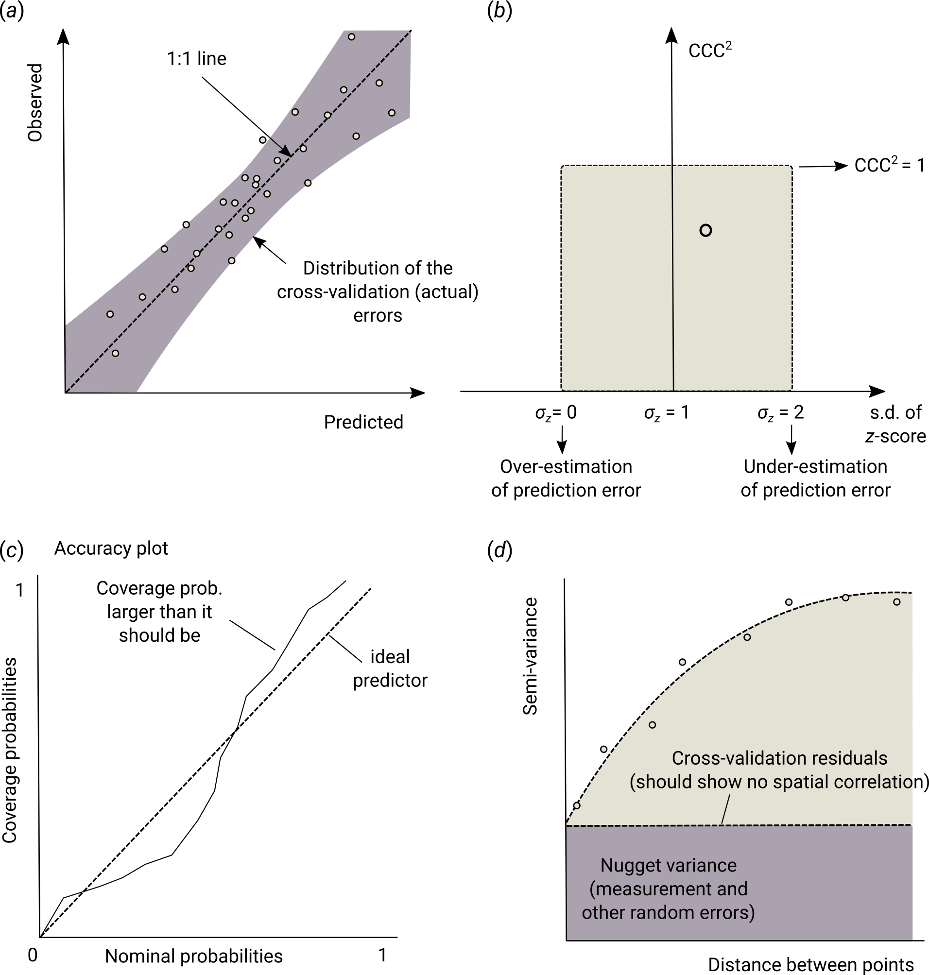
Figure 5.25: Universal plots of predictive performance: (a) 1:1 predicted vs observed plot, (b) CCC vs standard deviation of the z-scores plot, (c) nominal vs coverage probabilities, and (d) variogram of cross-validation residuals. Image source: Hengl et al. (2018) doi: 10.7717/peerj.5518.
So in summary, universal measures to access predicitive success of any spatial prediction method are (Hengl, Nussbaum, et al. 2018):
- Concordance Correlation Coefficient (0–1): showing predictive success of a method on a 1:1 predictions vs observations plot,
- Variance of the z-scores (0–\(\infty\)): showing how reliable the modeled estimate of the prediction errors is,
- Variogram of the cross-validation residuals: showing whether residuals still contain spatial dependence structure,
- Accuracy plots: showing whether the model over- or under-estimates either lower or higher values,
5.3.7 Mapping accuracy and soil survey costs
Once the accuracy of some model have been assessed, the next measure of overall mapping success of interest is the soil information production costs. Undoubtedly, producing soil information costs money. Burrough, Beckett, and Jarvis (1971), Bie and Ulph (1972), and Bie, Uph, and Beckett (1973) postulated in the early 70s that the survey costs are a direct function of the mapping scale:
\[\begin{equation} \log \begin{Bmatrix} {\rm cost} \; {\rm per} \; {\rm km}^2\\ {\rm or}\\ {\rm man-days} \; {\rm per} \; {\rm km}^2 \end{Bmatrix} = a + b \cdot \log( {\rm map} \; {\rm scale} ) \tag{5.35} \end{equation}\]To produce soil information costs money. On the other hand soil information, if used properly, can lead to significant financial benefits: accurate soil information is a tool to improve decision making, increase crop and livestock production and help to reduce investments risk and planning for environmental conservation.
This model typically explains >75% of the survey costs (Burrough, Beckett, and Jarvis 1971). Further more, for the given target scale, standard soil survey costs can be commonly expressed as:
\[\begin{equation} \theta = \frac{{\rm X}}{A} \qquad [{\rm USD} \; {\rm km}^{-2} ] \tag{5.36} \end{equation}\]where \({\rm X}\) is the total costs of a survey, \(A\) is the size of area in km-square. So for example, according to Legros (2006, 75), to map 1 hectare of soil at 1:200,000 scale (at the beginning of the 21st century), one needs at least 0.48 Euros (i.e. 48 EUR to map a square-km); to map soil at 1:20 would cost about 25 EUR per ha. These are the all-inclusive costs that include salaries and time in the office needed for the work of synthesis and editing.
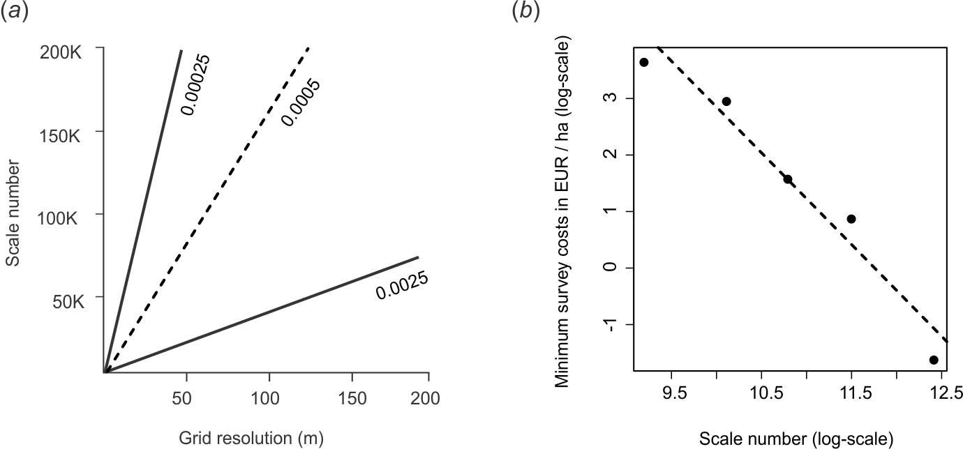
Figure 5.26: Some basic concepts of soil survey costs: (a) relationship between cartographic scale and pixel size (Hengl, 2006), (b) soil survey costs and scale relationship based on the empirical data of (Legros, 2006).
Estimated standard soil survey costs per area differ from country to country. The USDA estimates that the total costs of soil mapping at their most detailed scale (1:20) are about 1.50 USD per acre i.e. about 4 USD per ha (Durana 2008); in Canada, typical costs of producing soil maps at 1:20 are in the range 3–10 CAD per ha (MacMillan et al. 2010); in the Netherlands 3.4 EUR per ha (B. Kempen 2011, 149–54); in New Zealand 4 USD per ha (Carrick, Vesely, and Hewitt 2010). Based on these national-level numbers, Hengl, Nikolić, and MacMillan (2013) undertook to produce a global estimate of soil survey costs. So for example, to map 1 hectare of land at 1:20 scale, one would need (at least) 5 USD, and to map soil at 1:200,000 scale globally would cost about 8 USD per square-kilometer using conventional soil mapping methods.
A scale of 1:200,000 corresponds approximately to a ground resolution of 100 m (Fig. 5.26). If we would like to open a call to map the world’s soils (assuming that total land area to map is about 104 millions of square-km) using contemporary methods at 100 m resolution, and if we would consider 8 USD per square-kilometer as a reasonable cost, then the total costs for mapping the total productive soil areas of the world would be about 872 million USD. Of course, many countries in the world have already been mapped at a scale of 1:200,000 or finer, so this number could be reduced by at least 30%, but even then we would still need a considerable budget. This is just to illustrate that soil mapping can cost an order of magnitude more than, for example, land cover mapping.
Producing soil information costs money, but it also leads to financial benefits. Pimentel (2006) for example shows that the costs of soil erosion, measured just by the cost of replacing lost water and nutrients, is on the order of 250 billion USD annually. Soil information, if used properly, can also lead to increased crop and livestock production. Carrick, Vesely, and Hewitt (2010), for example, show that soil survey that costs (only) 3.99 USD per hectare, can lead to better management practices that help retain nitrogen in the soil at a rate of 42.49 USD per kg (17.30 USD per kg for farmers, 25.19 USD per kg for the community). This also demonstrates that soil mapping can be a profitable business.
The formula in Eq.(5.36) is somewhat incomplete as it tells us only about the cost of mapping per unit area. Obviously, mapping efficiency has to be expressed within the context of the mapping objective. Hence, a more informative measure of mapping efficiency is (Hengl, Nikolić, and MacMillan 2013):
\[\begin{equation} \theta = \frac{{\rm X}}{{A \cdot {\Sigma}_{\%}}} \qquad [{\rm USD} \; {\rm km}^{-2} \; \%^{-1} ] \tag{5.37} \end{equation}\]where \({\Sigma}_{\%}\) is the amount of variation explained by the spatial prediction model (Eq.(5.31)). In other words, soil mapping efficiency is the total cost of explaining each percent of variation in target soil variables for a given area of interest.
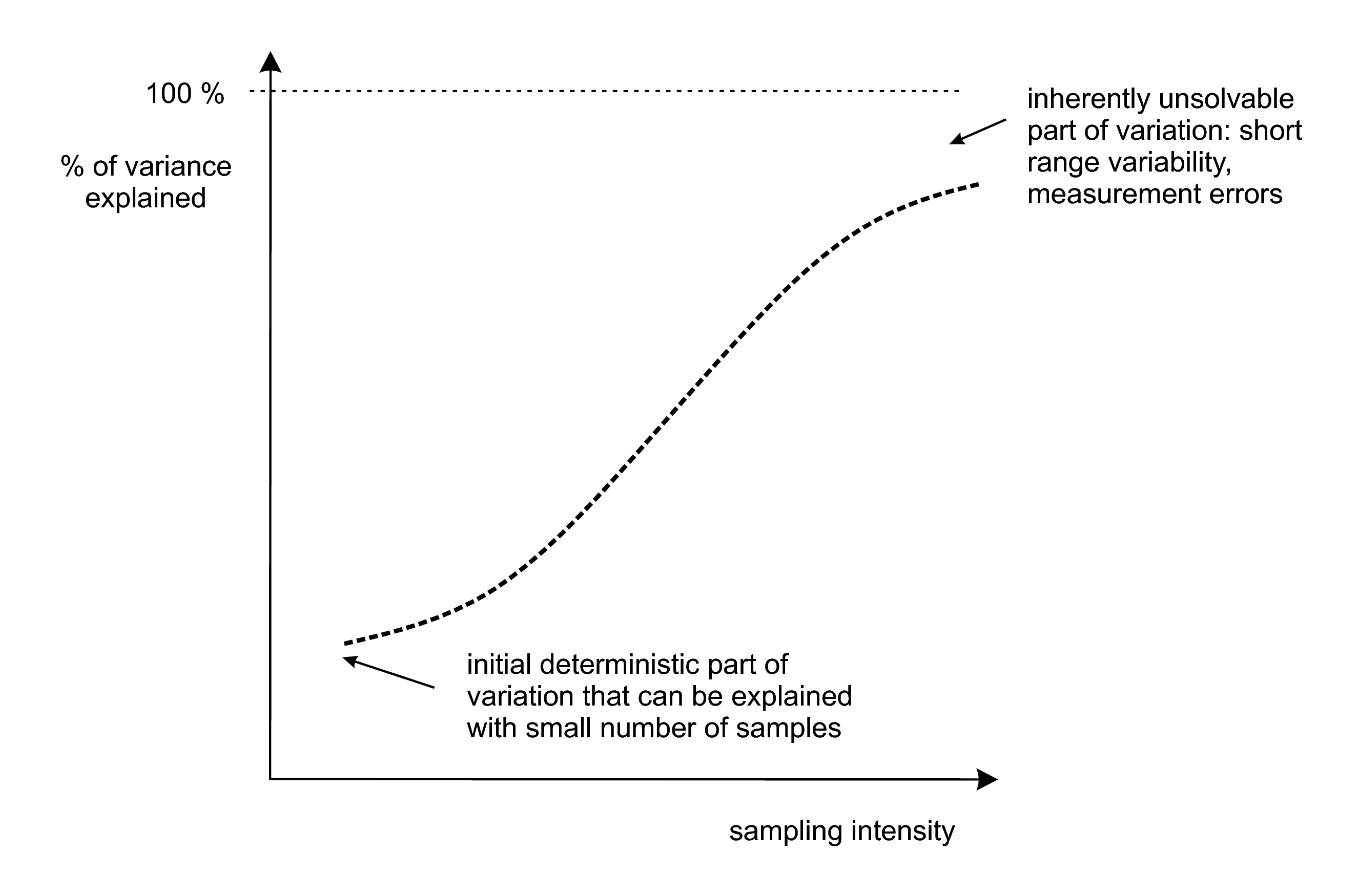
Figure 5.27: General relationship between the sampling intensity (i.e. survey costs) and amount of variation in the target variable explained by a spatial prediction model. After Hengl et al. (2013) doi: 10.1016/j.jag.2012.02.005.
An even more universal measure of mapping efficiency is the Information Production Efficiency (IPE) (Hengl, Nikolić, and MacMillan 2013):
\[\begin{equation} \Upsilon = \frac{{\rm X}}{{\rm gzip}} \qquad [{\rm EUR} \; {\rm B}^{-1}] \tag{5.38} \end{equation}\]where \({\rm gzip}\) is the size of data (in Bytes) left after compression and after recoding the values to match the effective precision (\(\delta \approx {\rm RMSE}/2\)). Information Production Efficiency is scale independent as the area is not included in the equation and hence can be used to compare the efficiency of various different soil mapping projects.
5.3.8 Summary points
Soil mapping processes are increasingly being automated, which is mainly due to advances in software for statistical computing and growing processing speed and computing capacity. Fully automated geostatistical mapping, i.e. generation of spatial predictions with little to no human interaction, is today a growing field of geoinformation science (Pebesma et al. 2011; P. E. Brown 2015; Hengl et al. 2014). Some key advantages of using automated soil mapping versus more conventional, traditional expert-based soil mapping are (Heuvelink et al. 2010; Bivand, Pebesma, and Rubio 2013):
All rules required to produce outputs are formalized. The whole procedure is documented (the statistical model and associated computer script), enabling reproducible research.
Predicted surfaces can make use of various information sources and can be optimized relative to all available quantitative point and covariate data.
There is more flexibility in terms of the spatial extent, resolution and support of requested maps.
Automated mapping is more cost-effective: once the system is operational, maintenance and production of updates are an order of magnitude faster and cheaper. Consequently, prediction maps can be updated and improved at shorter and shorter time intervals.
Spatial prediction models typically provide quantitative measures of prediction uncertainty (for each prediction location), which are often not provided in the case of conventional soil mapping.
A disadvantage of automated soil mapping is that many statistical and machine learning techniques are sensitive to errors and inconsistencies in the input data. A few typos, misaligned spatial coordinates or misspecified models can create serious artifacts and reduce prediction accuracy, more so than with traditional methods. Also, fitting models using large and complex data sets can be time consuming and selection of the ‘best’ model is often problematic. Explicit incorporation of conceptual pedological (expert) knowledge, which can be important for prediction in new situations to address the above issues, can be challenging as well.
In contemporary soil mapping, traditional concepts such as soil map scale and size of delineations are becoming increasingly dated or secondary. The focus of contemporary soil mapping is on minimizing costs required to explain variation in the target variable, while support size of the output maps can be set by the user. The amount of variation explained by a given statistical model gradually increases with sampling intensity, until it reaches some physical limit and does not result in any further improvements. Short-range variability and measurement error, e.g. the portion of the variation that cannot be captured or expressed by the model, for many soil variables can be as great as 10–40% (Fig. 5.27).
A useful thing for soil mapping teams is to compare a list of valid competing models and plot the differences for comparison studies using what we call “predictograms” (as illustrated in Fig. 5.28). Such comparison studies permit us to determine the best performing, and most cost effective, pedometric method for an area of interest and a list of target variables.
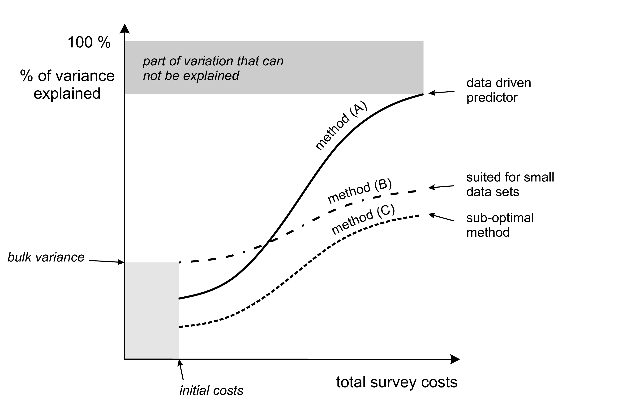
Figure 5.28: An schematic example of a performance plot (‘predictogram’) for comparing spatial prediction models. For more details see: Hengl et al. (2013) doi: 10.1016/j.jag.2012.02.005.
In summary, gauging the success of soil mapping basically boils down to the amount of variation explained by the spatial prediction model i.e. quantity of effective bytes produced for the data users. The survey costs are mainly a function of sampling intensity i.e. field work and laboratory data analysis. As we collect more samples for an area of interest we explain more and more of the total variance, until we reach some maximum feasible locked variation (Fig. 5.28). For a given total budget and a list of target variables an optimal (most efficient) prediction method can be determined by deriving the mapping efficiency described in Eq.(5.37) or even better Eq.(5.38).
By reporting on the RMSE, effective precision, information production efficiency, and by plotting the prediction variance estimated by the model, one gets a fairly good idea about the overall added information value in a given map. In other words, by assessing the accuracy of a map we can both recommend ways to improve the predictions (i.e. collect additional samples), and estimate the resources needed to reach some target accuracy. By assessing how the accuracy of various methods changes for various sampling intensities (Fig. 5.28), we can distinguish between methods that are more suited for particular regions, data sets or sizes of area and optimum methods that outperform all alternatives.
References
Finke, Peter A., and John L. Hutson. 2008. “Modelling Soil Genesis in Calcareous Loess.” Geoderma 145 (3-4):462–79. https://doi.org/10.1016/j.geoderma.2008.01.017.
Sommer, M., H.H. Gerke, and D. Deumlich. 2008. “Modelling Soil Landscape Genesis — a ‘Time Split’ Approach for Hummocky Agricultural Landscapes.” Geoderma 145 (3-4):480–93. https://doi.org/10.1016/j.geoderma.2008.01.012.
Minasny, Budiman, Alex B. McBratney, and S. Salvador-Blanes. 2008. “Quantitative Models for Pedogenesis — a Review.” Geoderma 144 (1-2):140–57. https://doi.org/10.1016/j.geoderma.2007.12.013.
Vanwalleghem, Tom, Jean Poesen, A McBratney, and J Deckers. 2010. “Spatial Variability of Soil Horizon Depth in Natural Loess-Derived Soils.” Geoderma 157 (1). Elsevier:37–45.
Hengl, T., G.B.M. Heuvelink, and D.G. Rossiter. 2007. “About Regression-Kriging: From Equations to Case Studies.” Computers & Geosciences 33 (10). Elsevier:1301–15.
Burrough, P. A., and R. A. McDonnell. 1998. Principles of Geographical Information Systems. 2nd ed. Oxford: Oxford University Press.
Webster, R., and M.A. Oliver. 2001. Geostatistics for Environmental Scientists. Statistics in Practice. Chichester: Wiley.
Matheron, G. 1969. Le krigeage universel. Vol. 1. Fontainebleau: Cahiers du Centre de Morphologie Mathématique, École des Mines de Paris.
Grunwald, S. 2005b. “What do we really know about the space-time continuum of soil-landscapes.” In Environmental Soil-Landscape Modeling: Geographic Information Technologies and Pedometrics, edited by S. Grunwald, 3–36. Boca Raton, Florida: CRC Press.
Desaules, André, Stefan Ammann, and Peter Schwab. 2010. “Advances in Long-Term Soil-Pollution Monitoring of Switzerland.” Journal of Plant Nutrition and Soil Science 173 (4). WILEY-VCH Verlag:525–35. https://doi.org/10.1002/jpln.200900269.
Snepvangers, J. J. J. C., G. B. M. Heuvelink, and J. A. Huisman. 2003. “Soil Water Content Interpolation Using Spatio-Temporal Kriging with External Drift.” Geoderma 112 (3). Elsevier:253–71.
Jost, G., G. B. M. Heuvelink, and A. Papritz. 2005. “Analysing the Space–Time Distribution of Soil Water Storage of a Forest Ecosystem Using Spatio-Temporal Kriging.” Geoderma 128 (3). Elsevier:258–73.
Gasch, Caley, Tomislav Hengl, Benedikt Gräler, Hanna Meyer, Troy Magney, and David Brown. 2015. “Spatio-temporal interpolation of soil water, temperature, and electrical conductivity in 3D+T: The Cook Agronomy Farm data set.” Spatial Statistics 14 (Part A):70–90. https://doi.org/10.1016/j.spasta.2015.04.001.
Kempen, B., D.J. Brus, and J.J. Stoorvogel. 2011. “Three-Dimensional Mapping of Soil Organic Matter Content Using Soil Type-Specific Depth Functions.” Geoderma 162 (1-2):107–23. https://doi.org/10.1016/j.geoderma.2011.01.010.
Bishop, T.F.A., A. B. McBratney, and G.M. Laslett. 1999. “Modelling Soil Attribute Depth Functions with Equal-Area Quadratic Smoothing Splines.” Geoderma 91 (1-2):27–45.
Malone, B.P., A. B. McBratney, B. Minasny, and G.M. Laslett. 2009. “Mapping Continuous Depth Functions of Soil Carbon Storage and Available Water Capacity.” Geoderma 154 (1-2):138–52. https://doi.org/10.1016/j.geoderma.2009.10.007.
Poggio, Laura, and Alessandro Gimona. 2014. “National scale 3D modelling of soil organic carbon stocks with uncertainty propagation — An example from Scotland.” Geoderma 232. Elsevier:284–99.
Hengl, Tomislav, Gerard B.M. Heuvelink, Bas Kempen, Johan G.B. Leenaars, Markus G. Walsh, Keith D. Shepherd, Andrew Sila, et al. 2015. “Mapping Soil Properties of Africa at 250 m Resolution: Random Forests Significantly Improve Current Predictions.” PLoS ONE 10 (e0125814). Public Library of Science. https://doi.org/10.1371/journal.pone.0125814.
Conant, Richard T, Stephen M Ogle, Eldor A Paul, and Keith Paustian. 2010. “Measuring and Monitoring Soil Organic Carbon Stocks in Agricultural Lands for Climate Mitigation.” Frontiers in Ecology and the Environment 9 (3). Ecological Society of America:169–73. http://dx.doi.org/10.1890/090153.
Baritz, Rainer, Guenther Seufert, Luca Montanarella, and Eric Van Ranst. 2010. “Carbon Concentrations and Stocks in Forest Soils of Europe.” Forest Ecology and Management 260:262–77. https://doi.org/10.1016/j.foreco.2010.03.025.
Panagos, Panos, Roland Hiederer, Marc Van Liedekerke, and Francesca Bampa. 2013. “Estimating soil organic carbon in Europe based on data collected through an European network.” Ecological Indicators 24 (0):439–50. https://doi.org/10.1016/j.ecolind.2012.07.020.
Cressie, N.A. C., and C.K. Wikle. 2011. Statistics for Spatio-Temporal Data. Wiley Series in Probability and Statistics. Wiley.
Ng, Wartini, Budiman Minasny, Brendan Malone, and Patrick Filippi. 2018. “In Search of an Optimum Sampling Algorithm for Prediction of Soil Properties from Infrared Spectra.” PeerJ 6 (October):e5722. https://doi.org/10.7717/peerj.5722.
Brus, D.J. 2019. “Sampling for digital soil mapping: A tutorial supported by R scripts.” Geoderma 338:464–80. https://doi.org/10.1016/j.geoderma.2018.07.036.
Diggle, P. J., and P. J. Ribeiro Jr. 2007. Model-based Geostatistics. Springer Series in Statistics. Springer.
Lark, RM, BR Cullis, and SJ Welham. 2006. “On spatial prediction of soil properties in the presence of a spatial trend: the empirical best linear unbiased predictor (E-BLUP) with REML.” European Journal of Soil Science 57 (6). Wiley Online Library:787–99.
McBratney, A. B., B. Minasny, R. A. MacMillan, and F. Carré. 2011. “Digital Soil Mapping.” In Handbook of Soil Science, edited by H. Li and M.E. Sumner, 37:1–45. CRC Press.
McBratney, A.B, M.L Mendonça Santos, and B Minasny. 2003. “On Digital Soil Mapping.” Geoderma 117 (1):3–52. https://doi.org/10.1016/S0016-7061(03)00223-4.
McBratney, A.B., B. Minasny, and U. Stockmann. 2018. Pedometrics. Progress in Soil Science. Springer International Publishing.
Li, Jin, and Andrew D. Heap. 2010. “A Review of Comparative Studies of Spatial Interpolation Methods in Environmental Sciences: Performance and Impact Factors.” Ecological Informatics 6 (3, 3-4). Elsevier:228–41. https://doi.org/10.1016/j.ecoinf.2010.12.003.
Schabenberger, O., and C. A. Gotway. 2005. Statistical Methods for Spatial Data Analysis. Texts in Statistical Science. Chapman & Hall/CRC.
de Gruijter, J.J., D.J. Brus, M.F.P. Bierkens, and M. Knotters. 2006. Sampling for Natural Resource Monitoring. London: Springer.
Pansu, M., J. Gautheyrou, and J.Y. Loyer. 2001. Soil Analysis: Sampling, Instrumentation and Quality Control. A.A. Balkema Publishers.
Tan, K.H. 2005. Soil Sampling, Preparation, and Analysis. Books in Soils, Plants, and the Environment. Taylor & Francis/CRC Press.
Legros, J.-P. 2006. Mapping of the Soil. 1st ed. Enfield, New Hampshire: Science Publishers.
Brus, D. J., and G. B. M. Heuvelink. 2007. “Optimization of sample patterns for universal kriging of environmental variables.” Geoderma 138 (1-2). Elsevier:86–95.
MacMillan, R. A., W. W. Pettapiece, and J. A. Brierley. 2005. “An Expert System for Allocating Soils to Landforms Through the Application of Soil Survey Tacit Knowledge.” Canadian Journal of Soil Science, 103–12.
Walter, C., P. Lagacherie, and S. Follain. 2006. “Integrating Pedological Knowledge into Digital Soil Mapping.” In Digital Soil Mapping — an Introductory Perspective, edited by P. Lagacherie, A. B. McBratney, and M. Voltz, 31:281–300, 615. Developments in Soil Science. Elsevier. https://doi.org/10.1016/S0166-2481(06)31022-7.
Liu, Jian, and A-Xing Zhu. 2009. “Mapping with words: A new approach to automated digital soil survey.” International Journal of Intelligent Systems 24 (3). Wiley Subscription Services, Inc., A Wiley Company:293–311. https://doi.org/10.1002/int.20337.
MacMillan, R.A., D.E. Moon, R.A. Coupé, and N. Phillips. 2010. “Predictive Ecosystem Mapping (Pem) for 8.2 Million Ha of Forestland,British Columbia, Canada.” In Digital Soil Mapping: Bridging Research, Environmental Application, and Operation, edited by J.L. Boettinger et al., 2:335–54. Progress in Soil Science. Springer. https://doi.org/10.1007/978-90-481-8863-5_27.
Simonson, Roy W. 1968. “Concept of Soil.” In Prepared Under the Auspices of the American Society of Agronomy, edited by A.G. Norman, 20:1–47. Advances in Agronomy. Academic Press. https://doi.org/10.1016/S0065-2113(08)60853-6.
Smith, G.D. 1986. The Guy Smith interviews: Rationale for Concepts in Soil Taxonomy. SMSS Technical Monograph No.11. Cornell University: Soil Management Support Services, USDA.
Mallavan, B.P., B. Minasny, and A. B. McBratney. 2010. “Homosoil, a Methodology for Quantitative Extrapolation of Soil Information Across the Globe.” In Digital Soil Mapping, edited by J. L. Boettinger, 2:137–49. Progress in Soil Science. Elsevier; Elsevier. https://doi.org/10.1007/978-90-481-8863-5_12.
Van Engelen, V.W.P., and J.A. Dijkshoorn, eds. 2012. Global and National Soils and Terrain Digital Databases (SOTER), Procedures Manual, version 2.0. ISRIC Report 2012/04. Wageningen, the Netherlands: ISRIC - World Soil Information.
Zhu, A.X., B. Hudson, J. Burt, K. Lubich, and D. Simonson. 2001. “Soil Mapping Using Gis, Expert Knowledge, and Fuzzy Logic.” Soil Science Society of America Journal 65:1463–72.
Zhu, A-Xing, Feng Qi, Amanda Moore, and James E. Burt. 2010. “Prediction of Soil Properties Using Fuzzy Membership Values.” Geoderma 158 (3-4):199–206. https://doi.org/10.1016/j.geoderma.2010.05.001.
Qi, Feng, A-Xing Zhu, Mark Harrower, and James E. Burt. 2006. “Fuzzy Soil Mapping Based on Prototype Category Theory.” Geoderma 136 (3-4):774–87. https://doi.org/10.1016/j.geoderma.2006.06.001.
Haining, Robert P., Ruth Kerry, and Margaret A. Oliver. 2010. “Geography, Spatial Data Analysis, and Geostatistics: An Overview.” Geographical Analysis 42 (1). Blackwell Publishing Inc:7–31. https://doi.org/10.1111/j.1538-4632.2009.00780.x.
Bivand, R., E. Pebesma, and V. Rubio. 2008. Applied Spatial Data Analysis with R. Use R Series. Heidelberg: Springer.
Hengl, T., J. Mendes de Jesus, G. B. M. Heuvelink, M. Ruiperez Gonzalez, M. Kilibarda, A. Blagotic, W. Shangguan, et al. 2017. “SoilGrids250m: Global Gridded Soil Information Based on Machine Learning.” PLoS One 12 (2):e0169748.
Hengl, Tomislav, Norair Toomanian, Hannes I. Reuter, and Mohammad J. Malakouti. 2007. “Methods to Interpolate Soil Categorical Variables from Profile Observations: Lessons from Iran.” Geoderma 140 (4). Elsevier:417–27. https://doi.org/10.1016/j.geoderma.2007.04.022.
Kempen, B., D.J. Brus, G.B.M. Heuvelink, and J.J. Stoorvogel. 2009. “Updating the 1:50,000 Dutch soil map using legacy soil data: A multinomial logistic regression approach.” Geoderma 151 (3-4):311–26. https://doi.org/10.1016/j.geoderma.2009.04.023.
Brown, Patrick E. 2015. “Model-Based Geostatistics the Easy Way.” Journal of Statistical Software 63 (12). http://www.jstatsoft.org/v63/i12.
Jenny, H., A. E. Salem, and J. R. Wallis. 1968. “Organic Matter and Soil Fertility.” In, edited by P. Salviucci, 32:5–36. Pontif. Acad. Sci. Scripta Varia. New York: North Holland Publishing Co., Amsterdam, & Wiley Interscience Division, John Wiley & Sons, Inc.
Jenny, H. 1994. Factors of Soil Formation: A System of Quantitative Pedology. Dover Books on Earth Sciences. Dover Publications.
Heuvelink, G.B.M., and R. Webster. 2001. “Modelling soil variation: past, present, and future.” Geoderma 100 (3-4).
Florinsky, I. V. 2012. “The Dokuchaev Hypothesis as a Basis for Predictive Digital Soil Mapping (on the 125th Anniversary of Its Publication).” Eurasian Soil Science 45 (4):445–51. https://doi.org/10.1134/S1064229312040047.
Kutner, M.H., J. Neter, C.J. Nachtsheim, and W. Li. 2005. Applied Linear Statistical Models. Operations and Decision Sciences Series. McGraw-Hill Irwin.
Yegnanarayana, B. 2004. Artificial Neural Networks. PHI Learning Pvt. Ltd.
Breiman, Leo. 1993. Classification and Regression Trees. CRC press.
Hearst, Marti A., S.T. Dumais, E. Osman, John Platt, and Bernhard Scholkopf. 1998. “Support Vector Machines.” Intelligent Systems and Their Applications, IEEE 13 (4). IEEE:18–28.
Breiman, Leo. 2001. “Random Forests.” Machine Learning 45 (1). Springer:5–32.
Meinshausen, Nicolai. 2006. “Quantile Regression Forests.” The Journal of Machine Learning Research 7 (Jun). JMLR.org:983–99.
Hastie, T.J., R.J. Tibshirani, and J.J.H. Friedman. 2009. The Elements of Statistical Learning: Data Mining, Inference, and Prediction. Springer Series in Statistics. Springer-Verlag New York.
Kuhn, Max, and Kjell Johnson. 2013. Applied Predictive Modeling. Vol. 810. Springer.
Statnikov, Alexander, Lily Wang, and Constantin Aliferis. 2008. “A Comprehensive Comparison of Random Forests and Support Vector Machines for Microarray-Based Cancer Classification.” BMC Bioinformatics 9 (1):319. https://doi.org/10.1186/1471-2105-9-319.
Kanevski, M., V. Timonin, and A. Pozdnukhov. 2009. Machine Learning for Spatial Environmental Data: Theory, Applications, and Software. Environmental Sciences. EFPL Press.
Lark, R.M., and A. Papritz. 2003. “Fitting a Linear Model of Coregionalization for Soil Properties Using Simulated Annealing.” Geoderma 115 (3). Elsevier:245–60.
Stein, M. L. 1999. Interpolation of Spatial Data: Some Theory for Kriging. Series in Statistics. New York: Springer.
Christensen, R. 2001. Linear Models for Multivariate, Time Series, and Spatial Data. 2nd ed. New York: Springer Verlag.
Venables, W. N., and B. D. Ripley. 2002. Modern applied statistics with S. 4th ed. New York: Springer-Verlag.
Goovaerts, P. 1997. Geostatistics for Natural Resources Evaluation (Applied Geostatistics). New York: Oxford University Press.
Yamamoto, JorgeKazuo. 2008. “Estimation or Simulation? That Is the Question.” Computational Geosciences 12 (4). Springer Netherlands:573–91. https://doi.org/10.1007/s10596-008-9096-8.
Kutner, M. H., C. J. Nachtsheim, J. Neter, and W. Li, eds. 2004. Applied Linear Statistical Models. 5th ed. McGraw-Hill.
Pebesma, Edzer J. 2004. “Multivariable geostatistics in S: the gstat package.” Computers & Geosciences 30 (7). Elsevier:683–91.
Bivand, R., E. Pebesma, and V. Rubio. 2008. Applied Spatial Data Analysis with R. Use R Series. Heidelberg: Springer.
2013. Applied Spatial Data Analysis with R. 2nd ed. Use R Series. Heidelberg: Springer.Pinheiro, J.C., and D. Bates. 2009. Mixed-Effects Models in S and S-PLUS. Statistics and Computing. Springer.
Minasny, B., and A.B. McBratney. 2001. “The Australian soil texture boomerang: A comparison of the Australian and USDA/FAO soil particle-size classification systems.” Australian Journal of Soil Research 39:1443–51.
2007. “Spatial prediction of soil properties using EBLUP with Matérn covariance function.” Geoderma 140:324–36.Kyriakidis, Phaedon C. 2004. “A Geostatistical Framework for Area-to-Point Spatial Interpolation.” Geographical Analysis 36 (3). Blackwell Publishing Ltd:259–89. https://doi.org/10.1111/j.1538-4632.2004.tb01135.x.
Hengl, T. 2006. “Finding the right pixel size.” Computers & Geosciences 32 (9):1283–98.
Heuvelink, G. B. M., and E. J. Pebesma. 1999. “Spatial aggregation and soil process modelling.” Geoderma 89 (1-2):47–65.
Hengl, T., M. Nikolić, and R. A. MacMillan. 2013. “Mapping Efficiency and Information Content.” International Journal of Applied Earth Observation and Geoinformation 22:127–38. https://doi.org/10.1016/j.jag.2012.02.005.
Heuvelink, G.B.M., and J. Brown. 2006. “Towards a Soil Information System for Uncertain Soil Data.” In Digital Soil Mapping: An Introductory Perspective, edited by P. Lagacherie, A. B. McBratney, and M. Voltz, 112–18. Developments in Soil Science. Amsterdam: Elsevier.
Heuvelink, G.B.M. 1998. Error Propagation in Environmental Modelling with Gis. London, UK: Taylor & Francis.
Brus, D.J., B. Kempen, and G.B.M. Heuvelink. 2011. “Sampling for Validation of Digital Soil Maps.” European Journal of Soil Science 62 (3). Blackwell Publishing Ltd:394–407. https://doi.org/10.1111/j.1365-2389.2011.01364.x.
Pebesma, Edzer, Dan Cornford, Gregoire Dubois, Gerard B.M. Heuvelink, Dionisis Hristopulos, Jürgen Pilz, Ulrich Stöhlker, Gary Morin, and Jon O. Skøien. 2011. “INTAMAP: The design and implementation of an interoperable automated interpolation web service.” Computers & Geosciences 37 (3). Elsevier:343–52. https://doi.org/10.1016/j.cageo.2010.03.019.
Brenning, A. 2012. “Spatial cross-validation and bootstrap for the assessment of prediction rules in remote sensing: The R package sperrorest.” In 2012 Ieee International Geoscience and Remote Sensing Symposium, 5372–5. https://doi.org/10.1109/IGARSS.2012.6352393.
Caubet, Manon, Mercedes Román Dobarco, Dominique Arrouays, Budiman Minasny, and Nicolas P.A. Saby. 2019. “Merging Country, Continental and Global Predictions of Soil Texture: Lessons from Ensemble Modelling in France.” Geoderma 337:99–110. https://doi.org/10.1016/j.geoderma.2018.09.007.
Heuvelink, G.B.M., and M.F.P. Bierkens. 1992. “Combining Soil Maps with Interpolations from Point Observations to Predict Quantitative Soil Properties.” Geoderma 55 (1-2):1–15. https://doi.org/10.1016/0016-7061(92)90002-O.
Mowrer, H. T., and R.G. Congalton. 2000. Quantifying spatial uncertainty in natural resources: theory and applications for GIS and remote sensing. Ann Arbor Press.
Goovaerts, Pierre. 2001. “Geostatistical Modelling of Uncertainty in Soil Science.” Geoderma 103 (1). Elsevier:3–26.
Finke, P. 2006. “Quality assessment of digital soil maps: producers and users perspectives.” In Digital Soil Mapping: An Introductory Perspective, edited by P. Lagacherie, A. B. McBratney, and M. Voltz, 523–41. Developments in Soil Science. Amsterdam: Elsevier.
Oreskes, Naomi, Kristin Shrader-Frechette, and Kenneth Belitz. 1994. “Verification, Validation, and Confirmation of Numerical Models in the Earth Sciences.” Science 263 (5147):641–46. https://doi.org/10.1126/science.263.5147.641.
Brodlie, Ken, Rodolfo Allendes Osorio, and Adriano Lopes. 2012. “A Review of Uncertainty in Data Visualization.” In Expanding the Frontiers of Visual Analytics and Visualization, 81–109. Springer.
Steichen, Thomas J, and Nicholas J Cox. 2002. “A Note on the Concordance Correlation Coefficient.” Stata J 2 (2):183–89.
Goovaerts, Pierre. 1999. “Geostatistics in Soil Science: State-of-the-Art and Perspectives.” Geoderma 89 (1). Elsevier:1–45.
Hengl, T., M. Nussbaum, M.N. Wright, G.B.M. Heuvelink, and B. Gräler. 2018. “Random Forest as a Generic Framework for Predictive Modeling of Spatial and Spatio-Temporal Variables.” PeerJ 6 (August):e5518. https://doi.org/10.7717/peerj.5518.
Burrough, P. A., P.H. T. Beckett, and M.G. Jarvis. 1971. “The Relation Between Cost and Utility in Soil Survey (I–Iii).” Journal of Soil Science 22 (3). Blackwell Publishing Ltd:359–94. https://doi.org/10.1111/j.1365-2389.1971.tb01624.x.
Bie, S.W., and A. Ulph. 1972. “The Economic Value of Survey Information.” Journal of Agricultural Economics 13:285–97.
Bie, S.W., A. Uph, and P.H. T. Beckett. 1973. “Calculating the Economic Benefits of Soil Survey.” Journal of Soil Science 24:429–35.
Durana, Patricia J. 2008. “Appendix A: Chronology of the U.S. Soil Survey.” In Profiles in the History of the U.S. Soil Survey, 315–20. Iowa State Press. https://doi.org/10.1002/9780470376959.app1.
Kempen, B. 2011. “Updating Soil Information with Digital Soil Mapping.” PhD thesis, Wageningen: Wageningen University. http://edepot.wur.nl/187198.
Carrick, Sam, Éva-Terézia Vesely, and Allan Hewitt. 2010. “Economic Value of Improved Soil Natural Capital Assessment: A Case Study on Nitrogen Leaching.” In 19th World Congress of Soil Science, 1–6. Brisbane, Australia: IUSS.
Pimentel, David. 2006. “Soil Erosion: A Food and Environmental Threat.” Environment, Development and Sustainability 8 (1). Kluwer Academic Publishers:119–37. https://doi.org/10.1007/s10668-005-1262-8.
Hengl, Tomislav, Jorge Mendes de Jesus, Robert A. MacMillan, Niels H. Batjes, Gerard B.M. Heuvelink, Eloi Ribeiro, Alessandro Samuel-Rosa, et al. 2014. “SoilGrids1km — Global Soil Information Based on Automated Mapping.” PLoS ONE 9 (e105992). Public Library of Science. https://doi.org/10.1371/journal.pone.0105992.
Heuvelink, GBM, DJ Brus, F De Vries, R Vašát, DJJ Walvoort, B Kempen, and M Knotters. 2010. “Implications of Digital Soil Mapping for Soil Information Systems.” In 4th Global Workshop on Digital Soil Mapping, Rome, 24–26.