4 Preparation of soil covariates for soil mapping
Edited by: T. Hengl and R. A. MacMillan
4.1 Soil covariate data sources
4.1.1 Types of soil covariates
Soils (and vegetation + ecosystems) form under complex interactions between climate, living organism and anthropogenic influences, modified by relief and hydrological processes and operating over long periods of time. This has been clearly identified first by Jenny (1994) with his CLORPT factors of soil formation and subsequently extended by McBratney, Mendonça Santos, and Minasny (2003) with the SCORPAN formulation (see section 1.3.3).
The following groups of covariates are commonly considered for use in Predictive Soil Mapping:
- Climate related covariates, which include:
- temperature maps,
- precipitation maps,
- snow cover maps,
- potential evapotranspiration,
- cloud fraction and other atmospheric images,
- Vegetation and living organisms, which include:
- vegetation indices e.g. FAPAR (mean, median), NDVI, EVI,
- biomass, Leaf Area Index,
- land cover type maps,
- vegetation types and communities (if mapped at high accuracy),
- land cover,
- Relief and topography-related covariates, which include:
- standard window-based calculations e.g. slope, curvatures, standard deviation,
- standard flow model outputs,
- landform classes / landform class likelihoods,
- hydrological / soil accumulation and deposition indices — MRVBFI, Wetness index, height above channel, height below ridge, horizontal distance to channel, horizontal distance to ridge,
- climatic and micro-climatic indices determined by relief e.g. incoming solar insolation and similar,
- Parent material / geologic material covariates, which include:
- bedrock type and age,
- bedrock mineralogy (acid, basic),
- surface material type, texture, age, mineralogy, thickness,
- volcanic activity, historic earthquake density,
- seismic activity level,
- gamma ray spectroscopy grids,
- gravity measurements,
- electrical conductivity/resistance,
- Estimated geological age of surface, which include:
- bedrock age / surface material age,
- recent disturbance age,
- Spatial position or spatial context, which include:
- latitude and longitude,
- distance to nearest large ocean
- Northing — distance to north pole,
- Southing — distance to south pole,
- Easting — distance to east,
- Westing — distance to west,
- shortest distance in any direction,
- distance to nearest high mountain,
- distance to nearest moderate hill,
- distance to nearest major river,
- Human or Anthropogenic Influences, which include:
- land use / land management maps,
- probability / intensity of agricultural land use,
- probability / intensity of pasture or grazing use,
- probability / intensity of forest land management,
- probability / intensity of urbanization,
- soil dredging, surface sealing,
- night time illumination (nightlights) images,
- probability of gullying or human-induced erosion,
- soil nutrient fertilization, liming and similar maps,
In the following sections we provide some practical advice (with links to the most important data sources) on how to prepare soil covariates for use in PSM.
4.1.2 Soil covariate data sources (30–100 m resolution)
Adding relevant covariates that can help explain the distribution of soil properties increases the accuracy of spatial predictions. Hence, prior to generating predictions of soil properties, it is a good idea to invest in preparing a list of Remote Sensing (RS), geomorphological/lithologic and DEM-based covariates that can potentially help explain the spatial distribution of soil properties and classes. There are now many finer resolution (30–250 m) covariates with global coverage that are publicly available without restrictions. The spatial detail, accessibility and accuracy of RS-based products has been growing exponentially and there is no evidence that this trend is going to slow down in the coming decades (Herold et al. 2016).
The most relevant (global) publicly available remote sensing-based covariates that can be downloaded and used to improve predictive soil mapping at high spatial resolutions are, for example:
SRTM and/or ALOS W3D Digital Elevation Model (DEM) at 30 m and MERIT DEM at 100 m (these can be used to derive at least 8–12 DEM derivatives of which some generally prove to be beneficial for mapping of soil chemical and hydrological properties);
Landsat 7, 8 satellite images, either available from USGS’s GloVis / EarthExplorer, or from the GlobalForestChange project repository (Hansen et al. 2013);
Landsat-based Global Surface Water (GSW) dynamics images at 30 m resolution for the period 1985–2016 (Pekel et al. 2016);
Global Land Cover (GLC) maps based on the GLC30 project at 30 m resolution for 2000 and 2010 (Chen et al. 2015) and similar land cover projects (Herold et al. 2016);
USGS’s global bare surface images at 30 m resolution;
JAXA’s ALOS (PALSAR/PALSAR-2) radar images at 20 m resolution (Shimada et al. 2014); radar images, bands HH: -27.7 (5.3) dB and HV: -35.8 (3.0) dB, from the JAXA’s ALOS project are especially interesting for mapping rock outcrops and exposed bedrock but are also used to distinguish between bare soil and dense vegetation;
Note that the required download time for 30 m global RS data can be significant if the data are needed for a larger area (hence you might consider using some RS data processing hub such as Sentinel hub, Google Earth Engine and/or Amazon Web Services instead of trying to download large mosaics yourself).
Most recently soil mappers can also use more advanced (commercial) remote sensing products often available at finer spatial resolution which include:
WorldDEM (https://worlddem-database.terrasar.com) at 12 m resolution multiband elevation products,
German hyperspectral satellite mission EnMAP (http://www.enmap.org) products, which have shown to be useful for mapping soil nutrients and minerals (Steinberg et al. 2016),
Sentinel-1 soil moisture products, currently limited to 1 km to 500 m resolutions but available at fast revisit times (Bauer-Marschallinger et al. 2019),
Hyperspectral imaging systems, similar to field-based soil spectroscopy, and the upcoming missions such as SHALOM (Italy and Israel), HypXIM (France) and HypsIRI (USA) will most likely revolutionaize use of remote sensing for soil mapping.
4.1.3 Soil covariate data sources (250 m resolution or coarser)
Hengl, Mendes de Jesus, et al. (2017) used a large stack of slightly coarser resolution covariate layers for producing SoilGrids250m predictions, most of which were based on remote sensing data:
DEM-derived surfaces — slope, profile curvature, Multiresolution Index of Valley Bottom Flatness (VBF), deviation from Mean Value, valley depth, negative and positive Topographic Openness and SAGA Wetness Index — all based on a global merge of SRTMGL3 DEM and GMTED2010 (Danielson and Gesch 2011). All DEM derivatives were computed using SAGA GIS (Conrad et al. 2015),
Long-term averaged monthly mean and standard deviation of the MODIS Enhanced Vegetation Index (EVI). Derived using a stack of MOD13Q1 EVI images (Savtchenko et al. 2004),
Long-term averaged mean monthly surface reflectances for MODIS bands 4 (NIR) and 7 (MIR). Derived using a stack of MCD43A4 images (Mira et al. 2015),
Long-term averaged monthly mean and standard deviation of the MODIS land surface temperature (daytime and nighttime). Derived using a stack of MOD11A2 LST images (Wan 2006),
Long-term averaged mean monthly hours under snow cover based on a stack of MOD10A2 8-day snow occurrence images (Hall and Riggs 2007),
Land cover classes (cultivated land, forests, grasslands, shrublands, wetlands, tundra, artificial surfaces and bareland cover) for the year 2010 based on the GlobCover30 product by the National Geomatics Center of China (Chen et al. 2015). Upscaled to 250 m resolution and expressed as percent of pixel coverage,
Monthly precipitation images derived as the weighted average between the WorldClim monthly precipitation (Hijmans et al. 2005) and GPCP Version 2.2 (Huffman and Bolvin 2009),
Long-term averaged mean monthly hours under snow cover. Derived using a stack of MOD10A2 8-day snow occurrence images,
Lithologic units (acid plutonics, acid volcanic, basic plutonics, basic volcanics, carbonate sedimentary rocks, evaporite, ice and glaciers, intermediate plutonics, intermediate volcanics, metamorphics, mixed sedimentary rocks, pyroclastics, siliciclastic sedimentary rocks, unconsolidated sediment) based on a Global Lithological Map GLiM (Hartmann and Moosdorf 2012),
Landform classes (breaks/foothills, flat plains, high mountains/deep canyons, hills, low hills, low mountains, smooth plains) based on the USGS’s Map of Global Ecological Land Units (Sayre et al. 2014).
Global Water Table Depth in meters (Fan, Li, and Miguez-Macho 2013),
Landsat-based estimated distribution of Mangroves (Giri et al. 2011),
Average soil and sedimentary-deposit thickness in meters (Pelletier et al. 2016).
The covariates above were selected to represent factors of soil formation according to Jenny (1994): climate, relief, living organisms, water dynamics and parent material. Of the five main factors, water dynamics and living organisms (especially vegetation dynamics) are not trivial to represent, as these operate over long periods of time and often exhibit chaotic behavior. Using reflectance bands such as the mid-infrared MODIS bands from a single day, would be of little use for soil mapping for areas with dynamic vegetation, i.e. with strong seasonal changes in vegetation cover. To account for seasonal fluctuation and for inter-annual variations in surface reflectance, long-term temporal signatures of the soil surface derived as monthly averages from long-term MODIS imagery (15 years of data) can be more effective to use (Hengl, Mendes de Jesus, et al. 2017). Long-term average seasonal signatures of surface reflectance or vegetation index provide a better indication of soil characteristics than only a single snapshot of surface reflectance. Computing temporal signatures of the land surface requires a considerable investment of time (comparable to the generation of climatic images vs temporary weather maps), but it is probably the best way to effectively represent the cumulative influence of living organisms on soil formation.
Behrens et al. (2018) recently reported that, for example, DEM derivatives derived at coarser resolutions correlated better with some targeted soil properties than the same derivatives derived at finer resolutions. In this case, resolution (or scale) was represented through various DEM aggregation levels and filter sizes. Some physical and chemical processes of soil formation or vegetation distribution might not be effective or obvious at finer aggregation levels, but these can become very visible at coarser aggregation levels. In fact, it seems that spatial dependencies and interactions of the covariates can often be explained better simply by aggregating DEM and its derivatives (Behrens et al. 2018).
4.2 Preparing soil covariate layers
Before we are able to fit spatial prediction models and generate soil maps, a significant amount of effort is first spent on preparing covariate “layers” that can be used as independent variables (i.e. “predictor variables”) in the statistical modelling. Typical operations used to generate soil covariate layers include:
Converting polygon maps to rasters,
Downscaling or upscaling (aggregating) rasters to match the target resolution (i.e. preparing a stack),
Filtering out missing pixels / reducing noise and multicolinearity (data overlap) problems,
Overlaying and subsetting raster stacks and points,
The following examples should provide some ideas about how to program these steps using the most concise possible syntax running the fastest and most robust algorithms. Raster data can often be very large (e.g. millions of pixels) so processing large stacks of remote sensing scenes in R needs to be planned carefully. The complete R tutorial can be downloaded from the github repository. Instructions on how to install and set-up all software used in this example can be found in the software installation chapter 2.
4.2.1 Converting polygon maps to rasters
Before we can attach a polygon map to other stacks of covariates, it needs to be rasterized i.e. converted to a raster layer defined with its bounding box (extent) and spatial resolution. Consider for example the Ebergötzen data set polygon map from the plotKML package (Fig. 4.1):
library(rgdal)
#> Loading required package: sp
#> rgdal: version: 1.3-6, (SVN revision 773)
#>  Geospatial Data Abstraction Library extensions to R successfully loaded
#>  Loaded GDAL runtime: GDAL 2.2.2, released 2017/09/15
#>  Path to GDAL shared files: /usr/share/gdal/2.2
#>  GDAL binary built with GEOS: TRUE
#>  Loaded PROJ.4 runtime: Rel. 4.8.0, 6 March 2012, [PJ_VERSION: 480]
#>  Path to PROJ.4 shared files: (autodetected)
#>  Linking to sp version: 1.3-1
library(raster)
library(plotKML)
#> plotKML version 0.5-9 (2019-01-04)
#> URL: http://plotkml.r-forge.r-project.org/
library(viridis)
#> Loading required package: viridisLite
data(eberg_zones)
spplot(eberg_zones[1])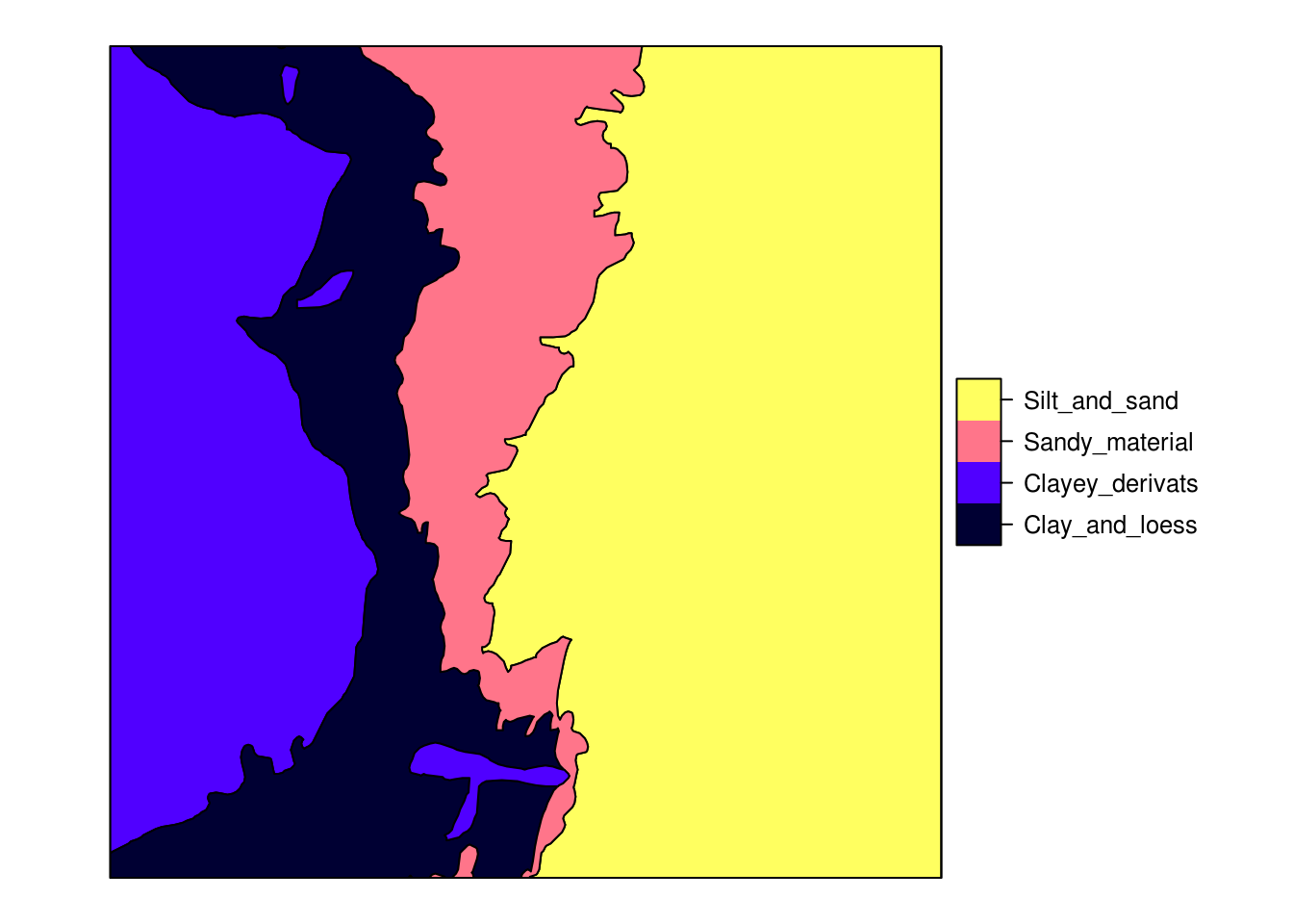
Figure 4.1: Ebergotzen parent material polygon map with legend.
We can convert this object to a raster by using the raster package. Note that before we can run the operation, we need to know the target grid system i.e. the extent of the grid and its spatial resolution. We can use this from an existing layer:
library(plotKML)
data("eberg_grid25")
gridded(eberg_grid25) <- ~x+y
proj4string(eberg_grid25) <- CRS("+init=epsg:31467")
r <- raster(eberg_grid25)
r
#> class       : RasterLayer
#> dimensions  : 400, 400, 160000  (nrow, ncol, ncell)
#> resolution  : 25, 25  (x, y)
#> extent      : 3570000, 3580000, 5708000, 5718000  (xmin, xmax, ymin, ymax)
#> coord. ref. : +init=epsg:31467 +proj=tmerc +lat_0=0 +lon_0=9 +k=1 +x_0=3500000 +y_0=0 +datum=potsdam +units=m +no_defs +ellps=bessel +towgs84=598.1,73.7,418.2,0.202,0.045,-2.455,6.7
#> data source : in memory
#> names       : DEMTOPx
#> values      : 159, 428  (min, max)
The eberg_grids25 object is a SpatialPixelsDataFrame, which is a spatial gridded data structure of the sp package package. The raster package also offers data structures for spatial (gridded) data, and stores such data as RasterLayer class. Gridded data can be converted from class SpatialPixelsDataFrame to a Raster layer with the raster command. The
CRS command of the sp package can be used to set a spatial projection.
EPSG projection 31467 is the German coordinate system (each coordinate system has an associated EPSG number that can be obtained from http://spatialreference.org/).
Conversion from polygon to raster is now possible via the rasterize command:
names(eberg_zones)
#> [1] "ZONES"
eberg_zones_r <- rasterize(eberg_zones, r, field="ZONES")
plot(eberg_zones_r)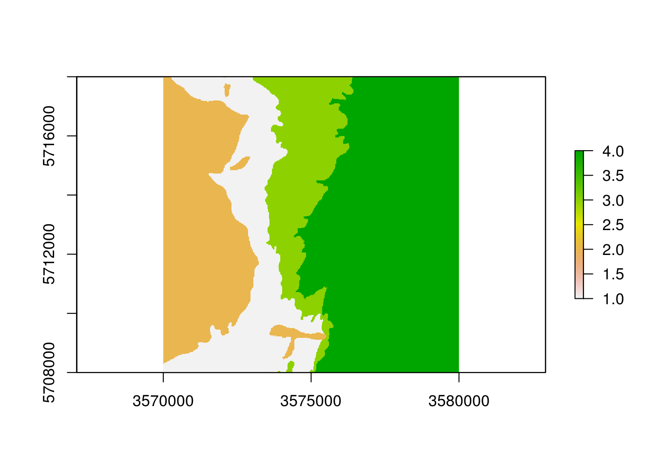
Figure 4.2: Ebergotzen parent material polygon map rasterized to 25 m spatial resolution.
Converting large polygons in R using the raster package can be very time-consuming. To speed up the rasterization of polygons we highly recommend using instead the fasterize function:
library(sf)
#> Linking to GEOS 3.5.0, GDAL 2.2.2, PROJ 4.8.0
library(fasterize)
#>
#> Attaching package: 'fasterize'
#> The following object is masked from 'package:graphics':
#>
#>     plot
eberg_zones_sf <- as(eberg_zones, "sf")
eberg_zones_r <- fasterize(eberg_zones_sf, r, field="ZONES")
fasterize function is an order of magnitude faster and hence more suitable for operational work; it only works with Simple Feature (sf) objects, however, so the sp polygon object needs to be first coerced to an sf object.
Another efficient approach to rasterize polygons is to use SAGA GIS, which can handle large data and is easy to run in parallel. First, you need to export the polygon map to shapefile format which can be done with commands of the rgdal package package:
eberg_zones$ZONES_int <- as.integer(eberg_zones$ZONES)
writeOGR(eberg_zones["ZONES_int"], "extdata/eberg_zones.shp", ".", "ESRI Shapefile")
The writeOGR() command writes a SpatialPolygonsDataFrame (the data structure for polygon data in R) to an ESRI shapefile. Here we only write the attribute "ZONES_int" to the shapefile. It is, however, also possible to write all attributes of the SpatialPolygonsDataFrame to a shapefile.
Next, you can locate the (previously installed) SAGA GIS command line program (on Microsoft Windows OS or Linux system):
if(.Platform$OS.type=="unix"){
  saga_cmd = "saga_cmd"
}
if(.Platform$OS.type=="windows"){
  saga_cmd = "C:/Progra~1/SAGA-GIS/saga_cmd.exe"
}
saga_cmd
#> [1] "saga_cmd"
and finally use the module grid_gridding to convert the shapefile to a grid:
pix = 25
system(paste0(saga_cmd, ' grid_gridding 0 -INPUT \"extdata/eberg_zones.shp\" ',
      '-FIELD \"ZONES_int\" -GRID \"extdata/eberg_zones.sgrd\" -GRID_TYPE 0 ',
      '-TARGET_DEFINITION 0 -TARGET_USER_SIZE ', pix, ' -TARGET_USER_XMIN ',
      extent(r)[1]+pix/2,' -TARGET_USER_XMAX ', extent(r)[2]-pix/2,
      ' -TARGET_USER_YMIN ', extent(r)[3]+pix/2,' -TARGET_USER_YMAX ',
      extent(r)[4]-pix/2))
#> Warning in system(paste0(saga_cmd, " grid_gridding 0 -INPUT \"extdata/
#> eberg_zones.shp\" ", : error in running command
eberg_zones_r2 <- readGDAL("extdata/eberg_zones.sdat")
#> extdata/eberg_zones.sdat has GDAL driver SAGA
#> and has 400 rows and 400 columns
With the system() command we can invoke an operating system (OS) command, here we use it to run the saga_cmd.exe file from R. The paste0 function is used to paste together a string that is passed to the system() command. The string starts with the OS command we would like to invoke (here saga_cmd.exe) followed by input required for the running the OS command.
Note that the bounding box (in SAGA GIS) needs to be defined using the center of the corner pixel and not the corners, hence we take half of the pixel size for extent coordinates from the raster package. Also note that the class names have been lost during rasterization (we work with integers in SAGA GIS), but we can attach them back by using e.g.:
levels(eberg_zones$ZONES)
#> [1] "Clay_and_loess"  "Clayey_derivats" "Sandy_material"  "Silt_and_sand"
eberg_zones_r2$ZONES <- as.factor(eberg_zones_r2$band1)
levels(eberg_zones_r2$ZONES) <- levels(eberg_zones$ZONES)
summary(eberg_zones_r2$ZONES)
#>  Clay_and_loess Clayey_derivats  Sandy_material   Silt_and_sand
#>           28667           35992           21971           73370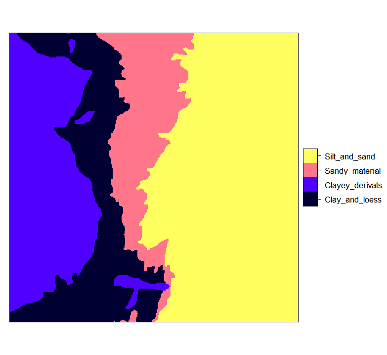
Figure 4.3: Ebergotzen zones rasterized to 25 m resolution and with correct factor labels.
4.2.2 Downscaling or upscaling (aggregating) rasters
In order for all covariates to perfectly stack, we also need to adjust the resolution of some covariates that have either too coarse or too fine a resolution compared to the target resolution. The process of bringing raster layers to a target grid resolution is also known as resampling. Consider the following example from the Ebergotzen case study:
data(eberg_grid)
gridded(eberg_grid) <- ~x+y
proj4string(eberg_grid) <- CRS("+init=epsg:31467")
names(eberg_grid)
#> [1] "PRMGEO6" "DEMSRT6" "TWISRT6" "TIRAST6" "LNCCOR6"
In this case we have a few layers that we would like to use for spatial prediction in combination with the maps produced in the previous sections, but their resolution is 100 m i.e. about 16 times coarser. Probably the most robust way to resample rasters is to use the gdalwarp function from the GDAL software. Assuming that you have already installed GDAL, you only need to locate the program on your system, and then you can again run gdalwarp via the system command:
writeGDAL(eberg_grid["TWISRT6"], "extdata/eberg_grid_TWISRT6.tif")
system(paste0('gdalwarp extdata/eberg_grid_TWISRT6.tif',
              ' extdata/eberg_grid_TWISRT6_25m.tif -r \"cubicspline\" -te ',
              paste(as.vector(extent(r))[c(1,3,2,4)], collapse=" "),
              ' -tr ', pix, ' ', pix, ' -overwrite'))
#> Warning in system(paste0("gdalwarp extdata/eberg_grid_TWISRT6.tif", "
#> extdata/eberg_grid_TWISRT6_25m.tif -r \"cubicspline\" -te ", : error in
#> running command
The writeGDAL command writes the TWISRT6 grid, that is stored in the eberg_grid grid stack, to a TIFF file. This TIFF is subsequently read by the gdalwarp function and resampled to a 25 m TIFF file using cubicspline, which will fill in values between original grid nodes using smooth surfaces. Note that the paste0 function in the system() command pastes together the following string:
"C:/Progra~1/GDAL/gdalwarp.exe eberg_grid_TWISRT6.tif
eberg_grid_TWISRT6_25m.tif -r \"cubicspline\"
-te 3570000 5708000 3580000 5718000 -tr 25 25 -overwrite"
We can compare the two maps (the original and the downscaled) next to each other by using:
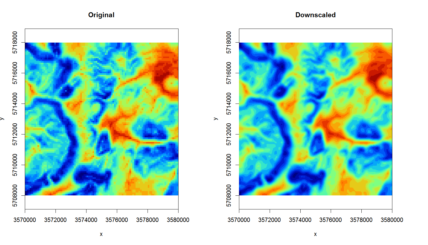
Figure 4.4: Original TWI vs downscaled map from 100 m to 25 m.
The map on the right looks much smoother of course (assuming that this variable varies continuously in space, this could very well be an accurate picture), but it is important to realize that downscaling can only be implemented up to certain target resolution i.e. only for certain features. For example, downscaling TWI from 100 to 25 m is not much of problem, but to go beyond 10 m would probably result in large differences from a TWI calculated at 10 m resolution (in other words: be careful with downscaling because it is often not trivial).
The opposite process to downscaling is upscaling or aggregation. Although this one can also potentially be tricky, it is a much more straightforward process than downscaling. We recommend using the average method in GDAL for aggregating values e.g.:
system(paste0('gdalwarp extdata/eberg_grid_TWISRT6.tif',
              ' extdata/eberg_grid_TWISRT6_250m.tif -r \"average\" -te ',
              paste(as.vector(extent(r))[c(1,3,2,4)], collapse=" "),
              ' -tr 250 250 -overwrite'))
#> Warning in system(paste0("gdalwarp extdata/eberg_grid_TWISRT6.tif", "
#> extdata/eberg_grid_TWISRT6_250m.tif -r \"average\" -te ", : error in
#> running command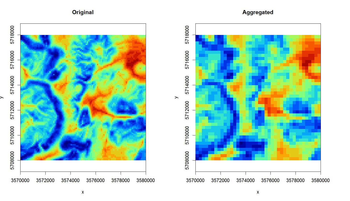
Figure 4.5: Original TWI vs aggregated map from 100 m to 250 m.
4.2.3 Deriving DEM parameters using SAGA GIS
Now that we have established a connection between R and SAGA GIS, we can also use SAGA GIS to derive some standard DEM parameters of interest to soil mapping. To automate further processing, we make the following function:
saga_DEM_derivatives <- function(INPUT, MASK=NULL,
                                 sel=c("SLP","TWI","CRV","VBF","VDP","OPN","DVM")){
  if(!is.null(MASK)){
    ## Fill in missing DEM pixels:
    suppressWarnings( system(paste0(saga_cmd,
                                    ' grid_tools 25 -GRID=\"', INPUT,
                                    '\" -MASK=\"', MASK, '\" -CLOSED=\"',
                                    INPUT, '\"')) )
  }
  ## Slope:
  if(any(sel %in% "SLP")){
    try( suppressWarnings( system(paste0(saga_cmd,
                                         ' ta_morphometry 0 -ELEVATION=\"',
                                         INPUT, '\" -SLOPE=\"',
                                         gsub(".sgrd", "_slope.sgrd", INPUT),
                                         '\" -C_PROF=\"',
                                         gsub(".sgrd", "_cprof.sgrd", INPUT), '\"') ) ) )
  }
  ## TWI:
  if(any(sel %in% "TWI")){
    try( suppressWarnings( system(paste0(saga_cmd,
                                         ' ta_hydrology 15 -DEM=\"',
                                         INPUT, '\" -TWI=\"',
                                         gsub(".sgrd", "_twi.sgrd", INPUT), '\"') ) ) )
  }
  ## MrVBF:
  if(any(sel %in% "VBF")){
    try( suppressWarnings( system(paste0(saga_cmd,
                                         ' ta_morphometry 8 -DEM=\"',
                                         INPUT, '\" -MRVBF=\"',
                                         gsub(".sgrd", "_vbf.sgrd", INPUT),
                                         '\" -T_SLOPE=10 -P_SLOPE=3') ) ) )
  }
  ## Valley depth:
  if(any(sel %in% "VDP")){
    try( suppressWarnings( system(paste0(saga_cmd,
                                         ' ta_channels 7 -ELEVATION=\"',
                                         INPUT, '\" -VALLEY_DEPTH=\"',
                                         gsub(".sgrd", "_vdepth.sgrd",
                                              INPUT), '\"') ) ) )
  }
  ## Openness:
  if(any(sel %in% "OPN")){
    try( suppressWarnings( system(paste0(saga_cmd,
                                         ' ta_lighting 5 -DEM=\"',
                                         INPUT, '\" -POS=\"',
                                         gsub(".sgrd", "_openp.sgrd", INPUT),
                                         '\" -NEG=\"',
                                         gsub(".sgrd", "_openn.sgrd", INPUT),
                                         '\" -METHOD=0' ) ) ) )
  }
  ## Deviation from Mean Value:
  if(any(sel %in% "DVM")){
    suppressWarnings( system(paste0(saga_cmd,
                                    ' statistics_grid 1 -GRID=\"',
                                    INPUT, '\" -DEVMEAN=\"',
                                    gsub(".sgrd", "_devmean.sgrd", INPUT),
                                    '\" -RADIUS=11' ) ) )
  }
}
To run this function we only need DEM as input:
writeGDAL(eberg_grid["DEMSRT6"], "extdata/DEMSRT6.sdat", "SAGA")
saga_DEM_derivatives("DEMSRT6.sgrd")
which processes all DEM derivatives at once. We can plot them using:
dem.lst <- list.files("extdata", pattern=glob2rx("^DEMSRT6_*.sdat"), full.names = TRUE)
plot(raster::stack(dem.lst), col=rev(magma(10, alpha = 0.8)))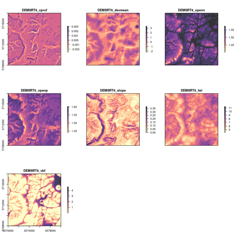
Figure 4.6: Some standard DEM derivatives calculated using SAGA GIS.
This function can now be used with any DEM to derive a standard set of 7–8 DEM parameters consisting of slope and curvature, TWI and MrVBF, positive and negative openness, valley depth and deviation from mean value. You could easily add more parameters to this function and then test if some of the other DEM derivatives can help improve mapping soil properties and classes. Note that SAGA GIS will by default optimize computing of DEM derivatives by using most of the available cores to compute (parallelization is turned on automatically).
4.2.4 Filtering out missing pixels and artifacts
After bringing all covariates to the same grid definition, remaining problems for using covariates in spatial modelling may include:
Missing pixels,
Artifacts and noise,
Multicolinearity (i.e. data overlap),
In a stack with tens of rasters, the weakest layer (i.e. the layer with greatest number of missing pixels or largest number of artifacts) could cause serious problems for producing soil maps as the missing pixels and artifacts would propagate to predictions: if only one layer in the raster stack misses values then predictive models might drop whole rows in the predictions even though data is available for 95% of rows. Missing pixels occur for various reasons: in the case of remote sensing, missing pixels can be due to clouds or similar; noise is often due to atmospheric conditions. Missing pixels (as long as we are dealing with only a few patches of missing pixels) can be efficiently filtered by using for example the gap filling functionality available in the SAGA GIS e.g.:
par(mfrow=c(1,2))
image(raster(eberg_grid["test"]), col=SAGA_pal[[1]], zlim=zlim, main="Original", asp=1)
image(raster("test.sdat"), col=SAGA_pal[[1]], zlim=zlim, main="Filtered", asp=1)
In this example we use the same input and output file for filling in gaps. There are several other gap filling possibilities in SAGA GIS including Close Gaps with Spline, Close Gaps with Stepwise Resampling and Close One Cell Gaps. Not all of these are equally applicable to all missing pixel problems, but having <10% of missing pixels is often not much of a problem for soil mapping.
Another elegant way to filter the missing pixels, to reduce noise and to reduce data overlap is to use Principal Components transformation of original data. This is available also via the GSIF function spc:
data(eberg_grid)
gridded(eberg_grid) <- ~x+y
proj4string(eberg_grid) <- CRS("+init=epsg:31467")
formulaString <- ~ PRMGEO6+DEMSRT6+TWISRT6+TIRAST6
eberg_spc <- GSIF::spc(eberg_grid, formulaString)
names(eberg_spc@predicted) # 11 components on the end;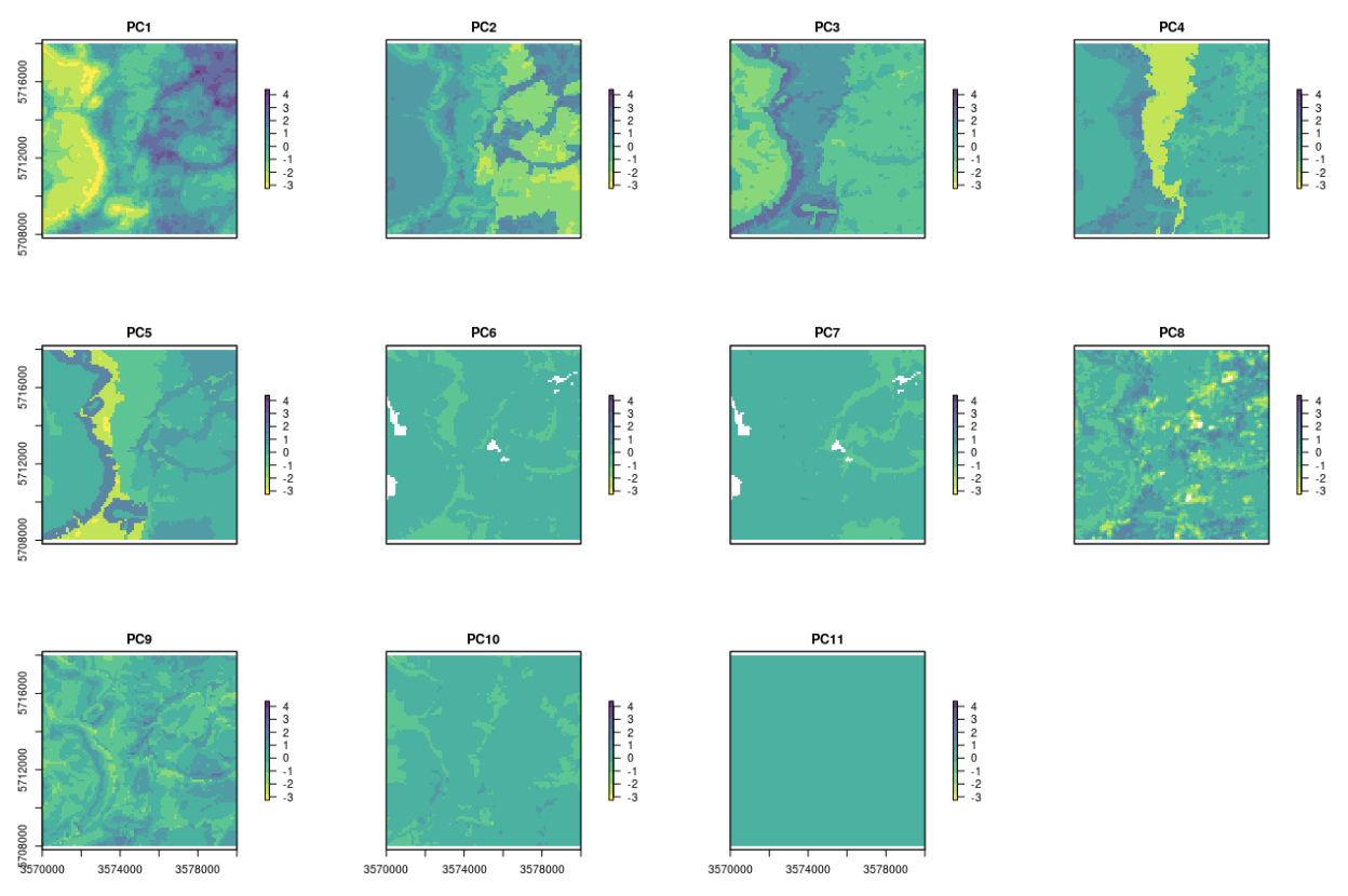
Figure 4.7: 11 PCs derived using input Ebergotzen covariates.
The advantages of using the spc function are:
All output soil covariates are numeric (and not a mixture of factors and numeric),
The last 1-2 PCs often contain signal noise and could be excluded from modelling,
In subsequent analysis it becomes easier to remove covariates that do not help in modelling (e.g. by using step-wise selection and similar),
A disadvantage of using spc is that these components are often abstract so that interpretation of correlations can become difficult. Also, if one of the layers contains many factor levels, then the number of output covariates might explode, which becomes impractical as we should then have at least 10 observations per covariate to avoid overfitting.
4.2.5 Overlaying and subsetting raster stacks and points
Now that we have prepared all covariates (resampled them to the same grid and filtered out all problems), we can proceed with running overlays and fitting statistical models. Assuming that we deal with a large number of files, an elegant way to read all those into R is by using the raster package, especially the stack and raster commands. In the following example we can list all files of interest, and then read them all at once:
library(raster)
grd.lst <- list.files(pattern="25m")
grd.lst
grid25m <- stack(grd.lst)
grid25m <- as(grid25m, "SpatialGridDataFrame")
str(grid25m)
One could now save all the prepared covariates stored in SpatialGridDataFrame as an RDS data object for future use.
saveRDS(grid25m, file = "extdata/covariates25m.rds")To overlay rasters and points and prepare a regression matrix, we can either use the over function from the sp package, or extract function from the raster package. By using the raster package, one can run overlay even without reading the rasters into memory:
library(sp)
data(eberg)
coordinates(eberg) <- ~X+Y
proj4string(eberg) <- CRS("+init=epsg:31467")
ov <- as.data.frame(extract(stack(grd.lst), eberg))
str(ov[complete.cases(ov),])
If the raster layers can not be stacked and if each layer is available in a different projection system, you can also create a function that reprojects points to the target raster layer projection system:
overlay.fun <- function(i, y){
  raster::extract(raster(i), na.rm=FALSE,
      spTransform(y, proj4string(raster(i))))}
which can also be run in parallel for example by using the parallel package:
ov  <- data.frame(mclapply(grd.lst, FUN=overlay.fun, y=eberg))
names(ov) <- basename(grd.lst)
In a similar way, one could also make wrapper functions that downscale/upscale grids, then filter missing values and stack all data together so that it becomes available in the working memory (sp grid or pixels object). Overlay and model fitting is also implemented directly in the GSIF package, so any attempt to fit models will automatically perform overlay.
4.2.6 Working with large(r) rasters
As R is often inefficient in handling large objects in memory (such as large raster images), a good strategy to run raster processing in R is to consider using for example the clusterR function from the raster package, which automatically parallelizes use of raster functions. To have full control over parallelization, you can alternatively tile large rasters using the getSpatialTiles function from the GSIF package and process them as separate objects in parallel. The following examples show how to run a simple function in parallel on tiles and then mosaic these tiles after all processing has been completed. Consider for example the sample GeoTiff from the rgdal package:
fn = system.file("pictures/SP27GTIF.TIF", package = "rgdal")
obj <- rgdal::GDALinfo(fn)
#> Warning in rgdal::GDALinfo(fn): statistics not supported by this driver
We can split that object in 35 tiles, each of 5 x 5 km in size by running:
tiles <- GSIF::getSpatialTiles(obj, block.x=5000, return.SpatialPolygons = FALSE)
tiles.pol <- GSIF::getSpatialTiles(obj, block.x=5000, return.SpatialPolygons = TRUE)
tile.pol  <- SpatialPolygonsDataFrame(tiles.pol, tiles)
plot(raster(fn), col=bpy.colors(20))
lines(tile.pol, lwd=2)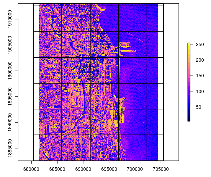
Figure 4.8: Example of a tiling system derived using the GSIF::getSpatialTiles function.
rgdal further allows us to read only a single tile of the GeoTiff by using the offset and region.dim arguments:
x = readGDAL(fn, offset=unlist(tiles[1,c("offset.y","offset.x")]),
             region.dim=unlist(tiles[1,c("region.dim.y","region.dim.x")]),
             output.dim=unlist(tiles[1,c("region.dim.y","region.dim.x")]), silent = TRUE)
spplot(x)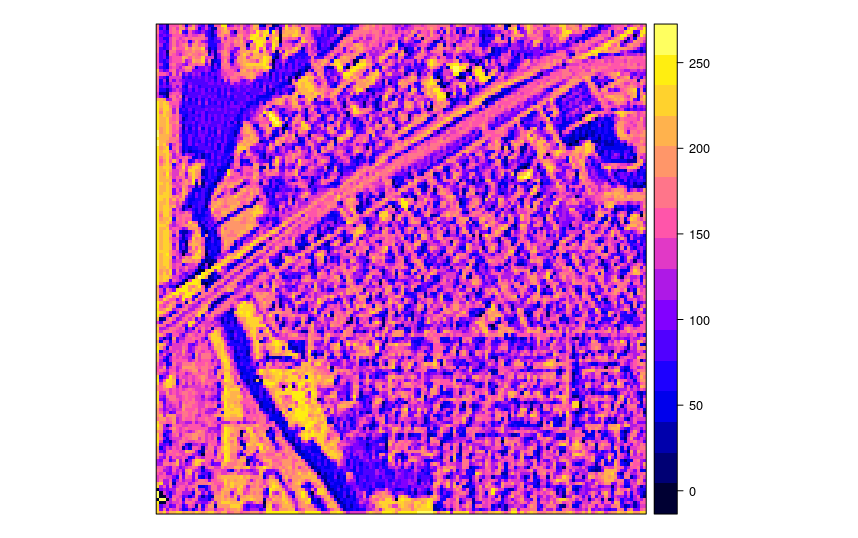
Figure 4.9: A tile produced from a satellite image in the example in the previous figure.
We would like to run a function on this raster in parallel, for example a simple function that converts values to 0/1 values based on a threshold:
fun_mask <- function(i, tiles, dir="./tiled/", threshold=190){
  out.tif = paste0(dir, "T", i, ".tif")
  if(!file.exists(out.tif)){
    x = readGDAL(fn, offset=unlist(tiles[i,c("offset.y","offset.x")]),
                 region.dim=unlist(tiles[i,c("region.dim.y","region.dim.x")]),
                 output.dim=unlist(tiles[i,c("region.dim.y","region.dim.x")]),
                 silent = TRUE)
    x$mask = ifelse(x$band1>threshold, 1, 0)
    writeGDAL(x["mask"], type="Byte", mvFlag = 255,
              out.tif, options=c("COMPRESS=DEFLATE"))
  }
}
This can now be run through the mclapply function from the parallel package (which automatically employs all available cores):
x0 <- mclapply(1:nrow(tiles), FUN=fun_mask, tiles=tiles)If we look in the tiles folder, this should show 35 newly produced GeoTiffs. These can be further used to construct a virtual mosaic by using:
t.lst <- list.files(path="extdata/tiled", pattern=glob2rx("^T*.tif$"),
                    full.names=TRUE, recursive=TRUE)
cat(t.lst, sep="\n", file="SP27GTIF_tiles.txt")
system('gdalbuildvrt -input_file_list SP27GTIF_tiles.txt SP27GTIF.vrt')
system('gdalwarp SP27GTIF.vrt SP27GTIF_mask.tif -ot \"Byte\"',
  ' -dstnodata 255 -co \"BIGTIFF=YES\" -r \"near\" -overwrite -co \"COMPRESS=DEFLATE\"')
Note we use a few important settings here for GDAL e.g.
-overwrite -co "COMPRESS=DEFLATE" to overwrite the GeoTiff and internally
compress it to save space, and -r "near" basically specifies that
no resampling is applied, just binding of tiles together. Also, if the
output GeoTiff is HUGE, you will most likely have to turn on -co "BIGTIFF=YES"
otherwise gdalwarp would not run through. The output mosaic looks like this:
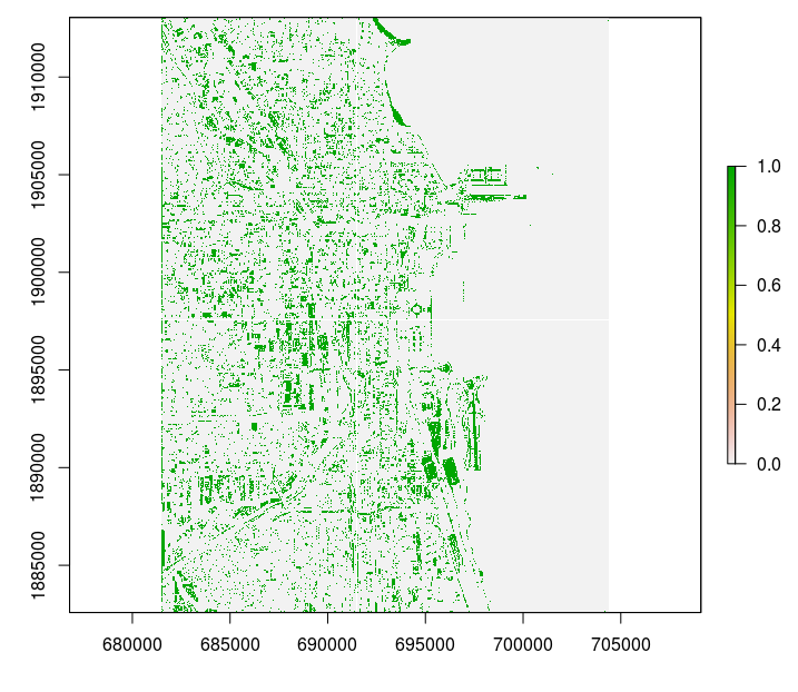
Figure 4.10: Final processed output.
This demonstrates that R can be used to compute with large rasters, provided
that these operations can be parallelized. Suggested best practice for this
is to: (1) design a tiling system that optimizes use of RAM and read/write
speed of a disk, (2) prepare and test a function that can then be run in
parallel, and (3) stitch back all tiles to create a single large raster
using gdalwarp.
Note that such tiling and stitching can not be applied universally to all problems e.g. functions that require global geographical search or all data in the raster. In such cases tiling should be applied with overlap (to minimize boundary effects) or to irregular tiling systems (e.g. per watershed). Once an optimal tiling system and function is prepared, R is no longer limited to running efficient computing, but only dependent on how much RAM and how many cores you have available i.e. it becomes more of a hardware than a software problem.
4.3 Summary points
Soil covariate layers are one of the key inputs to predictive soil mapping. Before any spatial layer can be used for modeling, it typically needs to be preprocessed to remove artifacts, resample to a standard resolution, fill in any missing values etc. All these operations can be successfully run by combining R and Open Source GIS software and by careful programming and optimization.
Preparing soil covariates can often be time and resources consuming so careful preparation and prioritization of processing is highly recommended. Hengl, Mendes de Jesus, et al. (2017) show that, for soil types and soil textures, DEM-parameters, i.e. soil forming factors of relief, especially flow-based DEM-indices, emerge as the second-most dominant covariates. These results largely correspond with conventional soil survey knowledge (surveyors have been using relief as a key guideline to delineate soil bodies for decades).
Although lithology is often not in the list of the top 15 most important predictors for PSM projects, spatial patterns of lithologic classes can often be distinctly recognized in the output predictions. This is especially true for soil texture fractions and coarse fragments. In general, for predicting soil chemical properties, climatic variables (especially precipitation) and surface reflectance seem to be the most important, while for soil classes and soil physical properties it is a combination of relief, vegetation dynamics and parent material. Investing extra time in preparing a better map of soil parent material is hence often a good idea.
Other potentially useful covariates for predicting soil properties and classes could be maps of paleo i.e. pre-historic climatic conditions of soil formation, e.g. glacial landscapes and processes, past climate conditions and similar. These could likely become significant predictors of many current soil characteristics. Information on pre-historic climatic conditions and land use is unfortunately often not available, especially not at detailed cartographic scales, although there are now several global products that represent, for example, dynamics of land use / changes of land cover (see e.g. HYDE data set (Klein Goldewijk et al. 2011)) through the past 1500+ years. As the spatial detail and completeness of such pre-historic maps increases, they will become potentially interesting covariates for global soil modeling.
USA’s NASA and USGS, with its SRTM, MODIS, Landsat, ICESat and similar civil-applications missions will likely remain the main source of spatial covariate data to support global and local soil mapping initiatives.
References
Jenny, H. 1994. Factors of Soil Formation: A System of Quantitative Pedology. Dover Books on Earth Sciences. Dover Publications.
McBratney, A.B, M.L Mendonça Santos, and B Minasny. 2003. “On Digital Soil Mapping.” Geoderma 117 (1):3–52. https://doi.org/10.1016/S0016-7061(03)00223-4.
Herold, Martin, Linda See, Nandin-Erdene Tsendbazar, and Steffen Fritz. 2016. “Towards an Integrated Global Land Cover Monitoring and Mapping System.” Remote Sensing 8 (12). https://doi.org/10.3390/rs8121036.
Hansen, M. C., P. V. Potapov, R. Moore, M. Hancher, S. A. Turubanova, A. Tyukavina, D. Thau, et al. 2013. “High-resolution global maps of 21st-century forest cover change.” Science 342 (6160). American Association for the Advancement of Science:850–53.
Pekel, Jean-François, Andrew Cottam, Noel Gorelick, and Alan S Belward. 2016. “High-Resolution Mapping of Global Surface Water and Its Long-Term Changes.” Nature 504. Nature Research:418–22.
Chen, Jun, Jin Chen, Anping Liao, Xin Cao, Lijun Chen, Xuehong Chen, Chaoying He, et al. 2015. “Global land cover mapping at 30 m resolution: A POK-based operational approach.” ISPRS Journal of Photogrammetry and Remote Sensing 103:7–27. https://doi.org/10.1016/j.isprsjprs.2014.09.002.
Shimada, Masanobu, Takuya Itoh, Takeshi Motooka, Manabu Watanabe, Tomohiro Shiraishi, Rajesh Thapa, and Richard Lucas. 2014. “New Global Forest/Non-Forest Maps from Alos Palsar Data (2007–2010).” Remote Sensing of Environment 155. Elsevier:13–31.
Steinberg, Andreas, Sabine Chabrillat, Antoine Stevens, Karl Segl, and Saskia Foerster. 2016. “Prediction of Common Surface Soil Properties Based on Vis-NIR Airborne and Simulated EnMAP Imaging Spectroscopy Data: Prediction Accuracy and Influence of Spatial Resolution.” Remote Sensing 8 (7). https://doi.org/10.3390/rs8070613.
Bauer-Marschallinger, B., V. Freeman, S. Cao, C. Paulik, S. Schaufler, T. Stachl, S. Modanesi, et al. 2019. “Toward Global Soil Moisture Monitoring With Sentinel-1: Harnessing Assets and Overcoming Obstacles.” IEEE Transactions on Geoscience and Remote Sensing 57 (1):520–39. https://doi.org/10.1109/TGRS.2018.2858004.
Hengl, T., J. Mendes de Jesus, G. B. M. Heuvelink, M. Ruiperez Gonzalez, M. Kilibarda, A. Blagotic, W. Shangguan, et al. 2017. “SoilGrids250m: Global Gridded Soil Information Based on Machine Learning.” PLoS One 12 (2):e0169748.
Danielson, J.J., and D.B. and Gesch. 2011. Global multi-resolution terrain elevation data 2010 (GMTED2010). Open-File Report 2011-1073. U.S. Geological Survey.
Conrad, O., B. Bechtel, M. Bock, H. Dietrich, E. Fischer, L. Gerlitz, J. Wehberg, V. Wichmann, and J. Böhner. 2015. “System for Automated Geoscientific Analyses (Saga) V. 2.1.4.” Geoscientific Model Development 8 (7). Copernicus GmbH:1991–2007. https://doi.org/10.5194/gmd-8-1991-2015.
Savtchenko, A., D. Ouzounov, S. Ahmad, J. Acker, G. Leptoukh, J. Koziana, and D. Nickless. 2004. “Terra and Aqua MODIS products available from NASA GES DAAC.” Advances in Space Research 34 (4):710–14. https://doi.org/10.1016/j.asr.2004.03.012.
Mira, Maria, Marie Weiss, Frédéric Baret, Dominique Courault, Olivier Hagolle, Belen Gallego-Elvira, and Albert Olioso. 2015. “The Modis (Collection V006) Brdf/Albedo Product Mcd43d: Temporal Course Evaluated over Agricultural Landscape.” Remote Sensing of Environment 170. Elsevier:216–28.
Wan, Zhengming. 2006. MODIS land surface temperature products users’ guide. ICESS, University of California.
Hall, Dorothy K, and George A Riggs. 2007. “Accuracy assessment of the MODIS snow products.” Hydrological Processes 21 (12). Wiley Online Library:1534–47.
Hijmans, R. J., S. E. Cameron, J. L. Parra, P. G. Jones, and A. Jarvis. 2005. “Very High Resolution Interpolated Climate Surfaces for Global Land Areas.” International Journal of Climatology 25:1965–78.
Huffman, George J, and David T Bolvin. 2009. GPCP version 2 combined precipitation data set documentation. Vol. 1. Laboratory for Atmospheres, NASA Goddard Space Flight Center; Science Systems; Applications.
Hartmann, Jens, and Nils Moosdorf. 2012. “The new global lithological map database GLiM: A representation of rock properties at the Earth surface.” Geochemistry, Geophysics, Geosystems 13 (12):n/a–n/a. https://doi.org/10.1029/2012GC004370.
Sayre, Roger, Jack Dangermond, Charlie Frye, Randy Vaughan, Peter Aniello, Sean Breyer, Douglas Cribbs, et al. 2014. A New Map of Global Ecological Land Units—an Ecophysiographic Stratification Approach. Washington, DC: USGS / Association of American Geographers.
Fan, Y, H Li, and G Miguez-Macho. 2013. “Global Patterns of Groundwater Table Depth.” Science 339 (6122). American Association for the Advancement of Science:940–43.
Giri, Chandra, E Ochieng, Larry L Tieszen, Z Zhu, Ashbindu Singh, T Loveland, J Masek, and Norm Duke. 2011. “Status and Distribution of Mangrove Forests of the World Using Earth Observation Satellite Data.” Global Ecology and Biogeography 20 (1). Wiley Online Library:154–59.
Pelletier, J. D., P. D. Broxton, P. Hazenberg, X. Zeng, P. A. Troch, G.-Y. Niu, Z. Williams, M. A. Brunke, and D. Gochis. 2016. “A Gridded Global Data Set of Soil, Immobile Regolith, and Sedimentary Deposit Thicknesses for Regional and Global Land Surface Modeling.” Journal of Advances in Modeling Earth Systems 8. https://doi.org/10.1002/2015MS000526.
Behrens, T., K. Schmidt, R.A. MacMillan, and R.A. Viscarra Rossel. 2018. “Multiscale Contextual Spatial Modelling with the Gaussian Scale Space.” Geoderma 310:128–37. https://doi.org/10.1016/j.geoderma.2017.09.015.
Klein Goldewijk, Kees, Arthur Beusen, Gerard Van Drecht, and Martine De Vos. 2011. “The Hyde 3.1 Spatially Explicit Database of Human-Induced Global Land-Use Change over the Past 12,000 Years.” Global Ecology and Biogeography 20 (1). Wiley Online Library:73–86.