1 Soil resource inventories and soil maps

Edited by: Hengl T. & MacMillan R.A.

1.1 Introduction

This chapter presents a description and discussion of soils and conventional soil inventories framed within the context of Predictive Soil Mapping (PSM). Soils, their associated properties, and their spatial and temporal distributions are the central focus of PSM. We discuss how the products and methods associated with conventional soil mapping relate to new, and emerging, methods of PSM and automated soil mapping. We discuss similarities and differences, strengths and weaknesses of conventional soil mapping (and its inputs and products) relative to PSM.

The universal model of soil variation presented in detail in Chapter 5 is adopted as a framework for comparison of conventional soil mapping and PSM. Our aim is to show how the products and methods of conventional soil mapping can complement, and contribute to, PSM and equally, how the theories and methods of PSM can extend and strengthen conventional soil mapping. PSM aims to implement tools and methods that can be supportive of growth, change and improvement in soil mapping and that can stimulate a rebirth and reinvigoration of soil inventory activity globally.

1.2 Soils and soil inventories

1.2.1 Soil: a definition

Soil is a natural body composed of biota and air, water and minerals, developed from unconsolidated or semi-consolidated material that forms the topmost layer of the Earth’s surface (Chesworth 2008). The upper limit of the soil is either air, shallow water, live plants or plant materials that have not begun to decompose. The lower limit is defined by the presence of hard rock or the lower limit of biologic activity (Richter and Markewitz 1995; Soil survey Division staff 1993). Although soil profiles up to tens of meters in depth can be found in some tropical areas (Richter and Markewitz 1995), for soil classification and mapping purposes, the lower limit of soil is often arbitrarily set to 2 m (http://soils.usda.gov/education/facts/soil.html). Soils are rarely described to depths beyond 2 m and many soil sampling projects put a primary focus on the upper (0-100 cm) depths.

The chemical, physical and biological properties of the soil differ from those of unaltered (unconsolidated) parent material from which the soil is derived over a period of time under the influence of climate, organisms and relief effects. Soil should show a capacity to support life, otherwise we are dealing with inert unconsolidated parent material. Hence, for purposes of developing statistically based models to predict soil properties using PSM, it proves useful to distinguish between actual and potential soil areas (see further section 1.4.4).

A significant aspect of the accepted definition of soil is that it is seen as a natural body that merits study, description, classification and interpretation in, and of, itself. As a natural body soil is viewed as an object that occupies space, has defined physical dimensions and that is more than the sum of its individual properties or attributes. This concept requires that all properties of soils be considered collectively and simultaneously in terms of a completely integrated natural body (Soil survey Division staff 1993). A consequence of this, is that one must generally assume that all soil properties covary in space in lockstep with specific named soils and that different soil properties do not exhibit different patterns of spatial variation independently relative to a named soil.

From a management point of view, soil can be seen from at least three perspectives. It is a:

  • Resource of materials — It contains quantities of unconsolidated materials, rock fragments, texture fractions, organic carbon, nutrients, minerals and metals, water and so on.

  • Stabilizing medium / ecosystem — It acts as a medium that supports both global and local processes from carbon and nitrogen fixation to retention and transmission of water, to provision of nutrients and minerals and so on.

  • Production system — Soil is the foundation for plant growth. In fact, it is the basis of all sustainable terrestrial ecosystem services. It is also a source of livelihood for people that grow crops and livestock.

For Frossard et al. (2006) there are six key functions of soil:

  1. food and other biomass production,

  2. storage, filtering, and transformation of water, gases and minerals,

  3. biological habitat and gene pool,

  4. source of raw materials,

  5. physical and cultural heritage and

  6. platform for man-made structures: buildings, highways.

Soil is the Earth’s biggest carbon store containing 82% of total terrestrial organic carbon (Lal 2004).

1.2.2 Soil variables

Knowledge about soil is often assembled and cataloged through soil resource inventories. Conventional soil resource inventories describe the geographic distribution of soil bodies i.e. polypedons (Wysocki, Schoeneberger, and LaGarry 2005). The spatial distribution of soil properties is typically recorded and described through reference to mapped soil individuals and not through separate mapping of individual soil properties. In fact, the definition of a soil map in the US Soil Survey Manual specifically “excludes maps showing the distribution of a single soil property such as texture, slope, or depth, alone or in limited combinations; maps that show the distribution of soil qualities such as productivity or erodibility; and maps of soil-forming factors, such as climate, topography, vegetation, or geologic material” (Soil survey Division staff 1993).

In contrast to conventional soil mapping, PSM is primarily interested in portraying, in the form of maps, the spatial distribution of soil variables — measurable or descriptive attributes commonly collected through field sampling and then either measured in-situ or a posteriori in laboratory. Soil variables can be roughly grouped into:

  1. quantities of some material (\(y \in [0 \rightarrow +\infty]\));

  2. transformed or standardized quantities such as pH (\(y \in [-\infty \rightarrow +\infty]\))

  3. relative percentages such as mass or volume percentages (\(y \in [0 \rightarrow 1]\));

  4. boolean values e.g. showing occurrence and/or non-occurrence of qualitative soil attributes or objects (\(y \in [0,1]\));

  5. categories (i.e. factors) such as soil classes (\(y \in [a,b,\ldots,x]\));

  6. probabilities e.g. probabilities of occurrence of some class or object (\(p(y) \in [0 \rightarrow 1]\)).

  7. censored values e.g. depth to bedrock which is often observed only up to 2 m.

The nature of a soil variable determines how the attribute is modeled and presented on a map in PSM. Some soil variables are normally described as discrete entities (or classes), but classes can also be depicted as continuous quantities on a map in the form of probabilities or memberships (de Gruijter, Walvoort, and Gaans 1997; A. B. McBratney, Mendoça Santos, and Minasny 2003; Kempen et al. 2009; Odgers, McBratney, and Minasny 2011). For example, a binary soil variable (e.g. the presence/absence of a specific layer or horizon) can be modeled as a binomial random variable with a logistic regression model. Spatial prediction (mapping) with this model gives a map depicting (continuous) probabilities in the range of 0–1. These probabilities can be used to determine the most likely presence/absence of a class at each prediction location, resulting, then, in a discrete representation of the soil attribute variation.

In that context, the aims of most soil resource inventories consist of the identification, measurement, modelling, mapping and interpretation of soil variables that represent transformed or standardized quantities of some material, relative percentages, occurrence and/or non-occurrence of qualitative attributes or objects, and/or soil categories.

1.2.3 Primary and secondary soil variables

Soil properties can be primary or inferred (see further section 3). Primary properties are properties that can be measured directly in the field or in the laboratory. Inferred properties are properties that cannot be measured directly (or are difficult or too expensive to measure) but can be inferred from primary properties, for example through pedotransfer functions (Wösten, Pachepsky, and Rawls 2001; Wösten et al. 2013). Dobos et al. (2006) also distinguish between primary and secondary soil properties and ‘functional’ soil properties representing soil functions or soil threats. Such soil properties can be directly used for financial assessment or for decision making. For example, soil organic carbon content in grams per kilogram of soil is the primary soil property, while organic carbon sequestration rate in kilograms per unit area per year is a functional soil property.

1.3 Soil mapping

1.3.1 What are soil resource inventories?

Soil resource inventories describe the types, attributes and geographic distributions of soils in a given area. They can consist of spatially explicit maps or of non-spatial lists. Lists simply itemize the kinds and amounts of different soils that occupy an area to address questions about what soils and soil properties occur in an area. The resulting answer is often not highly specific in space but rather presents a mainly non-spatial itemization of soils and soil attributes expected to occur in a bounded area. Maps attempt to portray, with some degree of detail, the patterns of spatial variation in soils and soil properties, within limits imposed by mapping scale and resources.

According to the USDA Manual of Soil Survey (Soil survey Division staff 1993), a soil survey:

  • describes the characteristics of the soils in a given area,

  • classifies the soils according to a standard system of classification,

  • plots the boundaries of the soils on a map, and

  • makes predictions about the behavior of soils.

The information collected in a soil survey helps in the development of land-use plans and evaluates and predicts the effects of land use on the environment. Hence, the different uses of the soils and how the response of management affects them need to be considered.

In conventional soil mapping, the objects of study, whose spatial distributions are portrayed on any resulting map, are soil individuals with each individual assumed to possess and exhibit a unique set of soil properties with a defined range of values. A fundamental assumption of conventional soil mapping is therefore that, if one maps the pattern of spatial distribution of uniquely defined soil individuals, one can infer the patterns of spatial distribution of the soil properties associated with each defined individual. Thus, conventional soil maps must, by definition, only map soil individuals and not individual soil properties (Soil survey Division staff 1993) and then subsequently infer the distribution of soil properties from the mapped distribution of soil individuals.

This attribute of conventional soil mapping represents a significant difference compared to PSM, where the object of study is frequently an individual soil property and the objective is to map the pattern of spatial distribution of that property (over some depth interval), often independently from consideration of the spatial distribution of soil individuals or other soil properties.

Soil maps give answers to three basic questions: (1) what is mapped?, (2) what is the predicted value?, and (3) where is it? Thematic accuracy of a map tells us how accurate predictions of targeted soil properties are overall, while the spatial resolution helps us locate features with some specified level of spatial precision.

The most common output of a soil resource inventory is a soil map. Soil maps convey information about the geographic distribution of named soil types in a given area. They are meant to help answer the questions “what is here” and “where is what” (Burrough and McDonnell 1998).

Any map is an abstraction and generalization of reality. The only perfect one-to-one representation of reality is reality itself. To fully describe reality one would need a model at 1:1 scale at which 1 m\(^2\) of reality was represented by 1 m\(^2\) of the model. Since this is not feasible, we condense and abstract reality in such a way that we hope to describe the major differences in true space at a much reduced scale in model (map) space. When this is done for soil maps, it needs to be understood that the map cannot describe all of the soil variation that is present in reality. It can only describe that portion of the total variation that is systematic and has structure and occurs over distances that are as large as, or larger than, the smallest area that can be feasibly portrayed and described at any given scale. Issues of scale and resolution are discussed in greater detail in chapter 4.2.2.

An important functionality of PSM is the production and distribution of maps depicting the spatial distribution of soils and, more specifically, soil attributes. In this chapter we, therefore, concentrate on describing processes for producing maps as spatial depictions of the patterns of arrangement of soil attributes and soil types.

1.3.2 Soil mapping approaches and concepts

As mentioned previously, spatial information about the distribution of soil properties or attributes, i.e. soil maps or GIS layers focused on soil, is produced through soil resource inventories, also known as soil surveys or soil mapping projects (Burrough, Beckett, and Jarvis 1971; Avery 1987; Wysocki, Schoeneberger, and LaGarry 2005; Legros 2006). The main idea of soil survey is, thus, production and dissemination of soil information for an area of interest usually to address a specific question or questions of interest i.e. production of soil maps and soil geographical databases. Although soil surveyors are usually not per se responsible for final use of soil information, how soil survey information is used is increasingly important.

In statistical terms, the main objective of soil mapping is to describe the spatial variability i.e. spatial complexity of soils, then represent this complexity using maps, summary measures, mathematical models and simulations. Some known sources of spatial variability in soil variables are:

  1. Natural spatial variability in 2D (different at various scales), mainly due to climate, parent material, land cover and land use;

  2. Variation by depth;

  3. Temporal variation due to regular or periodic changes in the ecosystem;

  4. Measurement error (in situ or in lab);

  5. Spatial location error;

  6. Small scale variation;

In statistical terms, the main objective of soil mapping is to describe the spatial complexity of soils, then represent this complexity using maps, summary measures, mathematical models and simulations. From the application point of view, the main application objective of soil mapping is to accurately predict response of a soil(-plant) ecosystem to various soil management strategies.

Soil mappers do their best to try explain the first two items above and minimize, or exclude from modelling, the remaining components: temporal variation, measurement error, spatial location error and small scale variation.

Inputs to soil-plant, soil-hydrology or soil-ecology models and their relationship.

Figure 1.1: Inputs to soil-plant, soil-hydrology or soil-ecology models and their relationship.

From the application point of view, the main objective of soil mapping is to accurately predict soil properties and their response to possible or actual management practices (Fig. 1.1). In other words, if the soil mapping system is efficient, we should be able to accurately predict the behavior of soil-plant, soil-hydrology or similar ecosystems to various soil management strategies, and hence provide useful advice to agronomists, engineers, environmental modelers, ecologists and similar.

We elect here to recognize two main variants of soil mapping which we refer to as conventional soil mapping and pedometric or predictive soil mapping as described and discussed below (Fig. 1.2).

Comparison between traditional (primarily expert-based) and automated (data-driven) soil mapping.

Figure 1.2: Comparison between traditional (primarily expert-based) and automated (data-driven) soil mapping.

1.3.3 Theoretical basis of soil mapping: in context of the universal model of spatial variation

Stated simply, “the scientific basis of soil mapping is that the locations of soils in the landscape have a degree of predictability” (Miller, McCormack, and Talbot 1979). According to the USDA Soil Survey Manual, “The properties of soil vary from place to place, but this variation is not random. Natural soil bodies are the result of climate and living organisms acting on parent material, with topography or local relief exerting a modifying influence and with time required for soil-forming processes to act. For the most part, soils are the same wherever all elements of these five factors are the same. Under similar environments in different places, soils are expected to be similar. This regularity permits prediction of the location of many different kinds of soil” (Soil survey Division staff 1993). Hudson (2004) considers that this soil-landscape paradigm provides the fundamental scientific basis for soil survey.

In the most general sense, both conventional soil mapping and PSM represent ways of applying the soil-landscape paradigm via the universal model of spatial variation, which is explained in greater detail in Chapter 5. Burrough and McDonnell (1998, 133) described the universal model of soil variation as a special case of the universal model of spatial variation. This model distinguishes between three major components of soil variation: (1) a deterministic component (trend), (2) a spatially correlated component and (3) pure noise.

\[\begin{equation} Z({\bf{s}}) = m({\bf{s}}) + \varepsilon '({\bf{s}}) + \varepsilon ''({\bf{s}}) \tag{1.1} \end{equation}\]

where \(\bf{s}\) is two-dimensional location, \(m({\bf{s}})\) is the deterministic component, \(\varepsilon '({\bf{s}})\) is the spatially correlated stochastic component and \(\varepsilon ''({\bf{s}})\) is the pure noise (micro-scale variation and measurement error).

The universal model of soil variation assumes that there are three major components of soil variation: (1) a deterministic component (function of covariates), (2) a spatially correlated component (treated as stochastic) and (3) pure noise.

The deterministic part of the equation describes that part of the variation in soils and soil properties that can be explained by reference to some model that relates observed and measured variation to readily observable and interpretable factors that control or influence this spatial variation. In conventional soil mapping, this model is the empirical and knowledge-based soil-landscape paradygm (Hudson 2004). In PSM, a wide variety of statistical, and machine learning, models have been used to capture and apply the soil-landscape paradigm in a quantitative and optimal fashion using the CLORPT model:

\[\begin{equation} S = f (cl, o, r, p, t) \tag{1.2} \end{equation}\]

where \(S\) stands for soil (properties and classes), \(cl\) for climate, \(o\) for organisms (including humans), \(r\) is relief, \(p\) is parent material or geology and \(t\) is time. The Eq. (1.2) is the CLORPT model originally presented by Jenny (1994).

A. McBratney, Mendonça Santos, and Minasny (2003) reconceptualized and extended the CLORPT model via the “scorpan” model in which soil properties are modeled as a function of:

  • (auxiliary) soil classes or properties,

  • climate,

  • oorganisms, vegetation or fauna or human activity,

  • relief,

  • parent material,

  • age i.e. the time factor,

  • n space, spatial conntext or spatial position,

Pedometric models are quantitative in that they capture relationships between observed soils, or soil properties, and controlling environmental influences (as represented by environmental co-variates) using statistically-formulated expressions. Pedometric models are seen as optimum because, by design, they minimize the variance between observed and predicted values at all locations with known values. So, no better model of prediction exists for that particular set of observed values at that specific set of locations.

Conventional soil mapping has a long history of effective development and application of empirical, knowledge-based, soil landscape models to predict how soil classes vary spatially across landscapes. Such models can be criticized, however, for being neither quantitative nor optimal.

Our essential point is that both conventional and pedometric soil mapping use models to explain the deterministic part of the spatial variation in soils and soil properties and these models differ mainly in terms of whether they are empirical and subjective (conventional) or quantitative and objective (pedometric). Both can be effective and the empirical and subjective models based on expert knowledge have, until recently, proven to be the most cost effective and widely applied for production of soil maps by conventional means.

The spatially correlated part of the observed variation is that part that shows spatial structure that lends itself to prediction through interpolation but that is not explainable, or easily explained, through use of a deterministic model that relates observed values to controlling environmental factors. This part of the variation is typically modeled in pedometric mapping using geostatistics and kriging to interpolate, in an optimal manner, between point locations with known values (Goovaerts 2001; A. B. McBratney, Mendoça Santos, and Minasny 2003).

It can be argued that conventional soil mapping has an analogue to kriging in situations where there is no clearly apparent relationship between observed values and readily observable controlling environmental variables. In such instances, conventional soil mappers typically resort to an approach in which they make as many closely spaced observations as feasible and then manually “interpolate” between these locations of known soils or soil properties to locate boundaries indicative of locations of significant change in soils or soil properties. In the vernacular of soil surveyors this is often referred to as “digging it out” in which a pattern that is not readily apparent or visible is revealed through interpolation between closely spaced observations. So, under some circumstances, conventional soil surveyors do implement an analogue of spatial interpolation to describe patterns of variation in soils where such patterns are not readily related to a clear soil-landscape model.

In its essence, the objective of PSM is to produce optimal unbiased predictions of a mean value at some new location along with the uncertainty associated with the prediction, at the finest possible resolution.

There is one way in which PSM differs significantly from conventional soil mapping in terms of the universal model of soil variation. This is in the use of geostatistics or machine learning to quantitatively correct for error in predictions, defined as the difference between predicted and observed values at locations with known values. Conventional soil mapping has no formal or quantitative mechanism for correcting an initial set of predicted values by computing the difference between predicted and observed values at sampled locations and then correcting initial values at all locations in response to these observed differences. PSM uses geostatistics to determine (via the semi-variogram) if the differences between predicted and observed values (the residuals) exhibit spatial structure (e.g. are predictable). If they do exhibit spatial structure, then it is useful and reasonable to interpolate the computed error at known locations to predict the likely magnitude of error of predictions at all locations (T. Hengl, Heuvelink, and Rossiter 2007). This interpolated prediction error can then be systematically subtracted from (or added to) the original predicted value to correct for errors in the initial predictions that are systematic and spatially correlated. This “after the fact” correction of initial predictions is an aspect of PSM that represents an improvement over conventional soil mapping methods and that conventional methods would do well to emulate.

Neither conventional soil mapping nor PSM can do more than simply describe and quantify the amount of variation that is not predictable and has to be treated as pure noise. Conventional soil maps can be criticized for ignoring this component of the total variation and typically treating it as if it did not exist. For many soil properties, short range, local variation in soil properties that cannot be explained by either the deterministic or stochastic components of the universal model of soil variation can often approach, or even exceed, a significant proportion (e.g. 30–40%) of the total observed range of variation in any given soil property. Such variation is simply not mappable but it exists and should be identified and quantified. We do our users and clients a disservice when we fail to alert them to the presence, and the magnitude, of spatial variation that is not predictable. In cases where the local spatial variation is not predictable (or mappable) the best estimate for any property of interest is the mean value for that local area or spatial entity.

1.3.4 Traditional (conventional) soil mapping

Traditional soil resource inventories are largely based on manual application of expert tacit knowledge through the soil-landscape paradigm (Burrough, Beckett, and Jarvis 1971; Hudson 2004). In this approach, soil surveyors develop and apply conceptual models of where and how soils vary in the landscape through a combination of field inspections to establish spatial patterns and photo-interpretation to extrapolate the patterns to similar portions of the landscape (Fig. 1.3). Traditional soil mapping procedures mainly address the deterministic part of the universal model of soil variation.

Typical soil survey phases and intermediate and final products.

Figure 1.3: Typical soil survey phases and intermediate and final products.

Conventional (traditional) manual soil mapping typically adheres to the following sequence of steps, with minor variations (A. B. McBratney, Mendoça Santos, and Minasny 2003):

  1. Specify the objective(s) to be served by the soil survey and resulting map;

  2. Identify which attributes of the soil or land need to be observed, described and mapped to meet the specified objectives;

  3. Identify the minimum sized area that must be described and the corresponding scale of mapping to meet the specified objectives;

  4. Collate and interpret existing relevant land resource information (geology, vegetation, climate, imagery) for the survey area;

  5. Conduct preliminary field reconnaissance and use these observations to construct a preliminary legend of conceptual mapping units (described in terms of soil individuals);

  6. Apply the preliminary conceptual legend using available source information to delineate initial map unit boundaries (pre-typing);

  7. Plan and implement a field program to collect samples and observations to obtain values of the target soil attributes (usually classes) at known locations to test and refine initial conceptual prediction models;

  8. Using field observations, refine the conceptual models and finalize map unit legends and boundaries to generate conventional area–class soil maps;

  9. Conduct a field correlation exercise to match mapping with adjacent areas and to confirm mapping standards were adhered to;

  10. Select and analyse representative soil profile site data to characterize each mapped soil type and soil map unit;

  11. Prepare final documentation that describes all mapped soils and soil map units (legends) according to an accepted format;

  12. Publish and distribute the soil information in the form of maps, geographical databases and reports;

Expert knowledge about soil-landform patterns is generally used to produce manually drawn polygon maps that outline areas of different dominant soils or combinations of soils — soil map units (see Figs. 1.4 and 1.10). Soil map units (polygons of different soil types) are described in terms of the composition of soil classes (and often also landscape attributes) within each unit, with various soil physical and chemical variables attached to each class. Most commonly, the objective of conventional soil mapping is to delineate recognizable portions of a landscape (soil–landform units) as polygons in which the variation of soils and soil properties is describable and usually (but not always) more limited than between polygons. Because most soil mapping projects have limited resources and time, soil surveyors can not typically afford to survey areas in great detail (e.g. 1:5000) so as to map actual polypedons. As a compromise, the survey team generally has to choose some best achievable target scale (e.g. 1:10,000 – 1:50,000). Maps produced at some initial scale can be further generalized, depending on the application and user demands (Wysocki, Schoeneberger, and LaGarry 2005).

Three basic conceptual scales in soil mapping: (left) most detailed scale showing the actual distribution of soil bodies, (center) target scale i.e. scale achievable by the soil survey budget, (right) generalized intermediate scale or coarse resolution maps. In a conventional soil survey, soils are described and conceptualized as groups of similar pedons (smallest elements of 1–10 square-m), called “polypedons” — the smallest mappable entity. These can then be further generalized to soil map units, which can be various combinations (systematic or random) of dominant and contrasting soils (inclusions).

Figure 1.4: Three basic conceptual scales in soil mapping: (left) most detailed scale showing the actual distribution of soil bodies, (center) target scale i.e. scale achievable by the soil survey budget, (right) generalized intermediate scale or coarse resolution maps. In a conventional soil survey, soils are described and conceptualized as groups of similar pedons (smallest elements of 1–10 square-m), called “polypedons” — the smallest mappable entity. These can then be further generalized to soil map units, which can be various combinations (systematic or random) of dominant and contrasting soils (inclusions).

Where variation within a polygon is systematic and predictable, the pattern of variation in soils within any given polygon is often described in terms of the most common position, or positions, in the landscape occupied by each named soil class MacMillan, Pettapiece, and Brierley (2005). In other cases, soil patterns are not clearly related to systematic variations in observable landscape attributes and it is not possible to describe where each named soil type is most likely to occur within any polygon or why.

Conventional soil mapping has some limitations related to the fact that mapping concepts (mental models) are not always applied consistently by different mappers. Application of conceptual models is largely manual and it is difficult to automate. In addition, conventional soil survey methods differ from country to country, and even within a single region, depending largely on the scope and level-of-detail of the inventory (Schelling 1970; Soil Survey Staff 1983; Rossiter 2003). The key advantages of conventional soil maps, on the other hand, are that:

  • they portray the spatial distribution of stable, recognizable and repeating patterns of soils that usually occupy identifiable portions of the landscape, and

  • these patterns can be extracted from legends and maps to model (predict) the most likely soil at any other location in the landscape using expert knowledge alone (Zhu et al. 2001).

Resource inventories, and in particular soil surveys, have been notoriously reluctant, or unable, to provide objective quantitative assessments of the accuracy of their products. For example, most soil survey maps have only been subjected to qualitative assessments of map accuracy through visual inspection and subjective correlation exercises. In the very few examples of quantitative evaluation (Marsman and de Gruijter 1986; Finke 2006), the assessments have typically focused on measuring the degree with which predictions of soil classes at specific locations on a map, or within polygonal areas on a map, agreed with on-the-ground assessments of the soil class at these same locations or within these same polygons. Measurement error can be large in assessing the accuracy of soil class maps. MacMillan et al. (2010), for example, demonstrated that experts disagreed with each other regarding the correct classification of ecological site types at the same locations about as often as they disagreed with the classifications reported by a map produced using a predictive model.

Assessments of map accuracy that compare the ability of a map to predict classes of soil at specific locations are insufficient to assess the ability of a map to predict spatial variation in soil properties. Maps are increasingly used to predict soil functional properties at specific (point) locations. In traditional soil mapping, all properties are tied to soil classes and all properties are assumed to vary in exactly the same manner as the observed variation in soil types. To predict the value of a soil property at a location, one would first predict the soil class most likely to occupy that location then infer the soil property based on the predicted soil class. This has disadvantages when soil properties do not covary exactly with soil classes and when spatial variation in soil classes is difficult to predict.

1.3.5 Variants of soil maps

In the last 20–30 years, soil maps have evolved from purely 2D polygon maps showing the distribution of soil poly-pedons i.e. named soil classes, to dynamic 3D maps representing predicted or simulated values of various primary or inferred soil properties and/or classes (Fig. 1.5). Examples of 2D+T and/or 3D+T soil maps are less common but increasingly popular (see e.g. Rosenbaum et al. (2012) and Gasch et al. (2015)). In general, we expect that demand for spatio-temporal soil data is likely to grow.

Classification of types of soil maps based on spatial representation and variable type.

Figure 1.5: Classification of types of soil maps based on spatial representation and variable type.

A soil map can represent 2D, 3D, 2D+T and/or 3D+T distribution of quantitative soil properties or soil classes. It can show predicted or simulated values of target soil properties and/or classes, or inferred soil-functions.

The spatial model increasingly used to represent soil spatial information is the gridded or raster data model, where most of the technical properties are defined by the grid cell size i.e. the ground resolution. In practice, vector-based polygon maps can be converted to gridded maps and vice versa, so in practical terms there are really few meaningful differences between the two models. In this book, to avoid any ambiguity, when mentioning soil maps we will often refer to the spatio-temporal reference and support size of the maps at the finest possible level of detail. Below, for example, is a full list of specifications attached to a soil map produced for the African continent (Hengl 2015):

  • target variable: soil organic carbon in permille;

  • values presented: predictions (mean value);

  • prediction method: 3D regression-kriging;

  • prediction depths: 6 standard layers (0–5, 5–15, 15–30, 30–60, 60–100, 100–200 cm);

  • temporal domain (period): 1950–2005;

  • spatial support (resolution) of covariate layers: 250 m;

  • spatial support of predictions: point support (center of a grid cell);

  • amount of variation explained by the spatial prediction model: 45%;

Until recently, maps of individual soil properties, or of soil functions or soil interpretations, were not considered to be true soil maps, but rather, to be single-factor derivative maps or interpretive maps. This is beginning to change and maps of the spatial pattern of distribution of individual soil properties are increasingly being viewed as a legitimate form of soil mapping.

1.3.6 Predictive and automated soil mapping

In contrast to traditional soil mapping, which is primarily based on applying qualitative expert knowledge, the emerging, ‘predictive’ approach to soil mapping is generally more quantitative and data-driven and based on the use of statistical methods and technology (Grunwald 2005a; Lagacherie, McBratney, and Voltz 2006; A. E. Hartemink, McBratney, and Mendonça-Santos 2008; Boettinger et al. 2010). The emergence of new soil mapping methods is undoubtedly a reflection of new developing technologies and newly available global data layers, especially those that are free and publicly distributed such as MODIS products, SRTM DEM and similar (Fig. 1.6). PSM can be compared to, and shares similar concepts with, other applications of statistics and machine learning in physical geography, for example Predictive Vegetation Mapping (Franklin 1995; T. Hengl, Walsh, et al. 2018).

Evolution of digital soil mapping parallels the emergence of new technologies and global, publicly available data sources.

Figure 1.6: Evolution of digital soil mapping parallels the emergence of new technologies and global, publicly available data sources.

The objective of using pedometric techniques for soil mapping is to develop and apply objective and optimal sets of rules to predict the spatial distribution of soil properties and/or soil classes. Most typically, rules are developed by fitting statistical relationships between digital databases representing the spatial distribution of selected environmental covariates and observed instances of a soil class or soil property at geo-referenced sample locations. The environmental covariate databases are selected as predictors of the soil attributes on the basis of either expert knowledge of known relationships to soil patterns or through objective assessment of meaningful correlations with observed soil occurrences. The whole process is amenable to complete automation and documentation so that it allows for reproducible research (read more in: http://en.wikipedia.org/wiki/Reproducibility).

Pedometric soil mapping typically follows six steps as outlined by A. B. McBratney, Mendoça Santos, and Minasny (2003):

  1. Select soil variables (or classes) of interest and suitable measurement techniques (decide what to map and describe);

  2. Prepare a sampling design (select the spatial locations of sampling points and define a sampling intensity);

  3. Collect samples in the field and then estimate values of the target soil variables at unknown locations to test and refine prediction models;

  4. Select and implement the most effective spatial prediction (or extrapolation) models and use these to generate soil maps;

  5. Select the most representative data model and distribution system;

  6. Publish and distribute the soil information in the form of maps, geographical databases and reports (and provide support to users);

Differences among conventional soil mapping, digital soil mapping or technology-driven or data-driven mapping relate primarily to the degree of use of robust statistical methods in developing prediction models to support the mapping process.

We here recognize four classes of soil mapping methods (B, C, D and E in Fig. 1.7) which all belong to a continuum of digital soil mapping methods (Malone, Minasny, and McBratney 2016; McBratney, Minasny, and Stockmann 2018). We promote in this book specifically the Class E soil mapping approach i.e. which we refer to as the predictive and/or automated soil mapping.

A classification of approaches to soil mapping: from purely expert driven (Class A), to various types of digital soil mapping including fully automated soil mapping (Class E).

Figure 1.7: A classification of approaches to soil mapping: from purely expert driven (Class A), to various types of digital soil mapping including fully automated soil mapping (Class E).

Some key advantages of the pedometric (statistical) approach to soil mapping are that it is: objective, systematic, repeatable, updatable and represents an optimal expression of statistically validated understanding of soil-environmental relationships in terms of the currently available data.

There are, of course, also limitations with pedometric methods that still require improvement. Firstly, the number of accurately georeferenced locations of reliable soil observations (particularly with analytical data) is often not sufficient to completely capture and describe all significant patterns of soil variation in an area. There may be too few sampled points and the exact location of available point data may not be well recorded. In short, data-driven soil mapping is field-data demanding and collecting field data can require significant expenditures of time, effort and money.

With legacy soil point data the sampling design, or rationale, used to decide where to locate soil profile observation or sampling points is often not clear and may vary from project to project or point to point. Therefore there is no guarantee that available point data are actually representative of the dominant patterns and soil forming conditions in any area. Points may have been selected and sampled to capture information about unusual conditions or to locate boundaries at points of transition and maximum confusion about soil properties. Once a soil becomes recognized as being widely distributed and dominant in the landscape, many conventional field surveys elect not to record observations when that soil is encountered, preferring to focus instead on recording unusual or transition soils. Thus the population of available legacy soil point observations may not be representative of the true population of soils, with some soils being either over or under-represented.

We define automated or predictive soil mapping as a data-driven approach to soil mapping with little or no human interaction, commonly based on using optimal (where possible) statistical methods that elucidate relationships between target soil variables (sampled in the field and geolocated) and covariate layers, primarily coming from remote sensing data.

A second key limitation of the automated approach to soil mapping is that there may be no obvious relationship between observed patterns of soil variation and the available environmental covariates. This may occur when a soil property of interest does, indeed, strongly covary with some mappable environmental covariate (e.g. soil clay content with airborne radiometric data) but data for that environmental covariate are not available for an area. It may also transpire that the pattern of soil variation is essentially not predictable or related to any known environmental covariate, available or not. In such cases, only closely spaced, direct field observation and sampling is capable of detecting the spatial pattern of variation in soils because there is no, or only a very weak, correlation with available covariates (Kondolf and Piégay 2003).

1.3.7 Comparison of conventional and pedometric or predictive soil mapping

There has been a tendency to view conventional soil mapping and automated soil mapping as competing and non-complementary approaches. In fact, they share more similarities than differences. Indeed, they can be viewed as end members of a logical continuum. Both rely on applying the underlying idea that the distribution of soils in the landscape is largely predictable (the deterministic part) and, where it is not predictable, it must be revealed through intensive observation, sampling and interpolation (the stochastic part).

In most cases, the basis of prediction is to relate the distribution of soils, or soil properties, in the landscape to observable environmental factors such as topographic position, slope, aspect, underlying parent material, drainage conditions, patterns of climate, vegetation or land use and so on. This is done manually and empirically (subjectively) in conventional soil survey, while in automated soil mapping it is done objectively and mostly in an automated fashion. At the time it was developed, conventional soil survey lacked both the digital data sets of environmental covariates and the statistical tools required to objectively analyze relationships between observed soil properties and environmental covariates. So, these relationships were, of necessity, developed empirically and expressed conceptually as expert knowledge.

More recently, it has become increasingly possible to obtain both environmental covariate data and field point soil observations in georegistered and digital format and to analyze and express relationships objectively and optimally, using statistical methods (Pebesma 2006; McBratney et al. 2011). Where the relationship between available environmental covariates and observed soil variation is weak, as in featureless plains or complex flood plains, both methods rely on similar approaches of using densely spaced point observations to reveal the spatial patterns. Conventional soil mappers ‘dig out’ these patterns while digital soil mappers interpolate using geostatistical procedures, but here too the two methods are quite analogous. Hard facts (point data and covariates) can often be beneficially enhanced using soft data (expert knowledge).

In general, we suggest that next generation soil surveyors will increasingly benefit from having a solid background in statistics and computer science, especially in Machine Learning and A.I. However, effective selection and application of appropriate statistical sampling and analysis techniques can also benefit from consideration of expert knowledge.

1.3.8 Top-down versus bottom-up approaches: subdivision versus agglomeration

There are two fundamentally different ways to approach the production of soil maps for areas of larger extent, whether by conventional or pedometric means. For ease of understanding we refer to these two alternatives here as “bottom-up” versus “top-down”. Rossiter (2003) refers to a synthetic approach that he calls the “bottom-up” or “name and then group” approach versus an analytic approach that he calls the “top-down” or “divide and then name” approach.

The bottom up approach is agglomerative and synthetic. It is implemented by first collecting observations and making maps at the finest possible resolution and with the greatest possible level of detail. Once all facts are collected and all possible soils and soil properties, and their respective patterns of spatial distribution, are recorded, these detailed data are generalized at successively coarser levels of generalization to detect, analyse and describe broader scale (regional to continental) patterns and trends. The fine detail synthesized to extract broader patterns leads to the identification and formulation of generalizations, theories and concepts about how and why soils organize themselves spatially. The bottom-up approach makes little, to no, use of generalizations and theories as tools to aid in the conceptualization and delineation of mapping entities. Rather, it waits until all the facts are in before making generalizations. The bottom-up approach tends to be applied by countries and organizations that have sufficient resources (people and finances) to make detailed field surveys feasible to complete for entire areas of jurisdiction. Soil survey activities of the US national cooperative soil survey (NCSS) primarily adopt this bottom-up approach. Other smaller countries with significant resources for field surveys have also adopted this approach (e.g. Netherlands, Denmark, Cuba). The bottom-up approach was, for example, used in the development and elaboration of the US Soil Taxonomy system of classification and of the US SSURGO (1:20,000) and STATSGO (1:250,000) soil maps (Zhong and Xu 2011).

The top-down approach is synoptic, analytic and divisive. It is implemented by first collecting just enough observations and data to permit construction of generalizations and theoretical concepts about how soils arrange themselves in the landscape in response to controlling environmental variables. Once general theories are developed about how environmental factors influence how soils arrange themselves spatially, these concepts and theories are tested by using them to predict what types of soils are likely to occur under similar conditions at previously unvisited sites. The theories and concepts are adjusted in response to initial application and testing until such time as they are deemed to be reliable enough to use for production mapping. Production mapping proceeds in a divisive manner by stratifying areas of interest into successively smaller, and presumably more homogeneous, areas or regions through application of the concepts and theories to available environmental data sets. The procedures begin with a synoptic overview of the environmental conditions that characterize an entire area of interest. These conditions are then interpreted to impose a hierarchical subdivision of the whole area into smaller, and more homogeneous subareas. This hierarchical subdivision approach owes its origins to early Russian efforts to explain soil patterns in terms of the geographical distribution of observed soils and vegetation. The top-down approach tends to be applied preferentially by countries and agencies that need to produce maps for very large areas but that lack the people and resources to conduct detailed field programs everywhere (see e.g. Henderson et al. (2004) and Mansuy et al. (2014)). Many of these divisive hierarchical approaches adopt principals and methods associated with the ideas of Ecological Land Classification (Rowe and Sheard 1981) (in Canada) or Land Systems Mapping (Gibbons, Downes, and others 1964; Rowan 1990) (in Australia).

As observed by Rossiter (2003) “neither approach is usually applied in its pure form” and most approaches to soil mapping use both approaches simultaneously, to varying degrees. Similarly, it can be argued that PSM provides support for both approaches to soil mapping. PSM implements two activities that bear similarities to bottom-up mapping. Firstly, PSM uses all available soil profile data globally as input to initial global predictions at coarser resolutions (“top-down” mapping). Secondly, PSM is set up to ingest finer resolution maps produced via detailed “bottom-up” mapping methods and to merge these more detailed maps with initial, coarser-resolution predictions (Ramcharan et al. 2018a).

1.4 Sources of soil data for soil mapping

1.4.1 Soil data sources targeted by PSM

PSM aims at integrating and facilitating exchange of global soil data. Most (global) soil mapping initiatives currently rely on capture and use of legacy soil data. This raises several questions. What is meant by legacy soil data? What kinds of legacy soil data exist? What are the advantages and limitations of the main kinds of legacy soil data?

In its most general sense, a legacy is something of value bequeathed from one generation to the next. It can be said that global soil legacy data consists of the sum of soil data and knowledge accumulated since the first soil investigations 100 or more years ago. More specifically, the concept of a legacy is usually accompanied by an understanding that there is an obligation and duty of the recipient generation to not simply protect the legacy but to make positive and constructive use of it.

The idea is that a legacy is not a priceless artifact, to be hidden away somewhere for static preservation and protection, but a living resource to be invested, improved upon, and grown for the sake of successive generations. The intention of any PSM framework is therefore not simply to rescue and protect the existing accumulation of legacy soil data, but to put it to new and beneficial uses, so that its value is increased and not just preserved.

Four main groups of legacy data of interest for global soil mapping are: (1) soil field records, (2) soil polygon maps and legends, (3) soil-landscape diagrams and sketches, (d) soil (profile) photographs.

In the context of soils, legacy soil data consist of the sum total of data, information and knowledge about soils accumulated since soils were first studied as independent natural objects. At its broadest, this includes information about soil characteristics and classification, soil use and management, soil fertility, soil bio-chemistry, soil formation, soil geography and many other subdisciplines.

In the more focused context of PSM, we are primarily interested in four main kinds of legacy soil data:

  • Soil field observations and measurements — Observations and analytical data obtained for soils at point locations represent a primary type of legacy soil data. These point source data provide objective evidence of observed soil characteristics at known locations that can be used to develop knowledge and rules about how soils, or individual soil properties, vary across the landscape. The quality and precision of these data can vary greatly. Some data points might be accurately located, or geo-referenced, while others might have very coarse geo-referencing (for example coordinates rounded in decimal minutes or kilometers). Some point data might only have a rough indication of the location obtained from a report (for example ‘2 km south of village A’), or might even lack geo-referencing. Soil profile descriptions can be obtained from pits (relatively accurate) or auger bores (less accurate). Soil attributes can be determined in the laboratory (relatively accurate) or by hand-estimation in the field (less accurate). Legacy point data is characterized by great variation in precision, accuracy, completeness, relevance and age. It needs to be used with caution and with understanding of how these issues affect its potential use.

  • Soil (polygon) maps and legends — Soil maps and legends are one of the primary means by which information and knowledge about how soils vary spatially have been observed, distilled, recorded and presented to users. Soil maps provide lists, or inventories, of soils that occur in mapped regions, illustrate the dominant spatial patterns displayed by these listed soils and provide information to characterize the main properties of these soils. Soil maps can themselves be used as sources of evidence to develop knowledge and quantitative rules about how soils, or individual soil properties, vary across the landscape. On the other hand, similar to soil observations, soil maps also can exhibit significant errors with respect to measurement, classification, generalization, interpretation and spatial interpolation.

  • Tacit expert soil knowledge — In the context of soils, tacit expert knowledge represents a diffuse domain of information about the characteristics and spatial distribution of soils that has not been captured and recorded formally or explicitly. It may reside in the minds and memories of experts who have conducted field and laboratory studies but have been unable to record all their observations in a formal way. It may be captured informally and partially in maps, legends, conceptual diagrams, block diagrams, generalized decision rules and so on. Tacit knowledge represents soft data, in comparison to the more hard data of point observations and maps.

  • Photographs — Traditional soil survey is heavily based on use of aerial photographs. Older aerial photographs (even if not stereoscopic) are an important resource for land degradation monitoring and vegetation succession studies. Field photographs of soil profiles, soil sites and soil processes are another important source of information that has been under-used for soil mapping. ISRIC for example has an archive of over 30 thousand photographs from various continents. Most of these can be geo-coded and distributed via image sharing web-services such as WikiMedia, Instagram and/or Flickr. In theory, even a single photograph of a soil profile could be used to (automatically?) identify soil types, even extract analytical soil properties. Although it is very likely that prediction by using photographs only would be fairly imprecise, such data could potentially help fill large gaps for areas where there are simply no soil observations.

1.4.2 Field observations of soil properties

Perhaps the most significant, certainly the most reliable, inputs to soil mapping are the field observations (usually at point locations) of descriptive and analytical soil properties (Soil survey Division staff 1993; Schoeneberger et al. 1998). This is the hard data or ground truth in soil mapping (Rossiter 2003). Field observations are also the main input to spatial prediction modelling and the basis for assessment of mapping accuracy. Other synthetically or empirically generated estimates of values of target variables in the field are considered as soft data. Soft data are less desirable as the primary input to model estimation, but sometimes there is no alternative. It is in any case important to recognize differences between hard and soft data and to suggest ways to access the uncertainty of models that are based on either or both.

The object of observation and description of a soil is almost always a soil profile or pedon. Officially, a soil pedon is defined as a body of soil having a limited horizontal extent of no more than 1–2 m in horizontal and a vertical dimension (\(d\)) that typically extends to only 1–2 m but may occasionally extend to greater depths. In practice, the vast majority of soil profile data pertain to soil observations and samples collected over very limited horizontal dimensions (10–50 cm) and down to maximum depths of 1–2 m.

In geostatistical terms, soil observations are most commonly collected at point support, meaning that they are representative of a point in space with very limited horizontal extent. It is relatively rare to encounter legacy soil profile data collected over larger horizontal extents and bulked to create a sample representative of a larger volume of soil that can be treated as providing block support for statistical purposes. On the other hand, there is an increasing interest in soil predictions at varying support sizes e.g. 1 ha for which composite sampling can be used.

In the vertical dimension, soil profiles are usually described and sampled with respect to genetic soil horizons, which are identifiable layers in the soil that reflect differences in soil development or depositional environments. Less frequently, soils are described and sampled in the vertical dimension with respect to arbitrary depth intervals or layers e.g. at fixed depths intervals e.g. 10, 20, 30, 40, \(\ldots\) cm.

A soil profile record is a set of field observations of the soil at a location — a collection of descriptive and analytical soil properties attached to a specific location, depth and sampling support size (volume of soil body).

Soil profile descriptions in the vertical dimension are usually accompanied by additional soil site descriptions that describe attributes of the site in the horizontal dimension for distances of a few meters to up 10 m to surrounding the location where the vertical profile was sampled and described. Site attributes described typically characterize the immediately surrounding landscape, including slope gradient, aspect, slope position, surface shape, drainage condition, land use, vegetation cover, stoniness and unusual or site specific features.

Two main types of information are typically recorded for point soil profiles. The first consists of field observations and classifications of observable profile and site characteristics. Profile attributes usually include the location and thickness of observably different horizons or layers, the color, texture, structure and consistence of each recognized horizon or layer and other observable attributes such as stone content, presence, size and abundance of roots, pores, mottles, cracks and so on. Despite their potential for subjectivity, these field observations provide much useful information at a relatively low cost, since there is no need to sample or transport the soil or analyze it at considerable cost in a distant laboratory.

The second main type of information collected to describe soil profiles consists of various types of objective measurements and analyses. Some objective measurements can be taken on-site, in the field. Examples of field measurements include in-situ assessment of bulk density, infiltration rate, hydraulic conductivity, electrical conductivity, penetration resistance and, more recently, spectral analysis of soil reflectance (Kondolf and Piégay 2003; Gehl and Rice 2007; Shepherd and Walsh 2007). The most frequently obtained and reported objective measurements are obtained by off-site laboratory analysis of soil samples collected from soil profiles at sampled locations. A wide variety of chemical and physical laboratory analyses can be, and have been, carried out on soil samples included in legacy soil profile data bases.

Within PSM we are mainly interested in a core set of laboratory analyses for e.g. pH, organic carbon, sand, silt, clay, coarse fragment content, bulk density, available water capacity, exchangeable cations and acidity and electrical conductivity. This core set was selected partly because it is considered to represent the key soil functional properties of most interest and use for interpretation and analysis and partly because these soil properties are the most widely analyzed and reported in the soil legacy literature (Sanchez et al. 2009; Hartemink et al. 2010). The significant feature of objective measurements is that they are expected to be consistent, repeatable and comparable across time and space. We will see in the following chapter that this is not always the case.

An advantage of descriptive field observations such as soil color, stone content, presence, size and abundance of roots, pores, mottles, cracks, diagnostic horizons etc. is that they provide much useful information at a relatively low cost, since there is no need to sample or transport the soil or analyze it at considerable cost in a distant laboratory.

1.4.3 Legacy soil profile data

The principal advantage of legacy soil profile data at point locations is simply that the observations and measurements are referenced to a known location in space (and usually also time). Knowledge of the spatial location of soil profile data provides the opportunity to analyze relationships between known data values at a location and other covariate (predictor) data sets. It also becomes possible to simply analyze spatial patterns i.e. represent spatial variability using values at known point locations. In the first instance, knowing the location of a point at which a soil property has been described or measured permits that location to be overlaid onto other spatially referenced digital data layers to produce data sets of related environmental values that all occur at the same site.

The known point values of soil properties (or classes) can be analyzed relative to the known values of environmental covariates at corresponding locations. If a statistically significant relationship can be established between the value of a soil property at numerous locations and the corresponding values of a environmental variables at the same locations, a predictive model can be developed. Development of predictive models based on such observed environmental correlations is a fundamental aspect of modern pedometric soil mapping.

A second main advantage of point profile data is that the data values are, more or less, objective assessments of a soil property or characteristic at a location. Objective values are more amenable to exploration using statistical techniques than subjective observations and classifications. They typically (but not always) exhibit less measurement error.

As important and useful as soil point data are, they also possess limitations and problems that must be recognized and addressed. One common limitation of legacy soil point data is lack of accurate geo-referencing information. The location information provided for older soil legacy profile data is often poor. Prior to the widespread adoption of the Global Positioning Systems (GPS) the locations of most soil sampling points were obtained and described in terms of estimated distances and directions from some known local reference point (Fig. 1.8). Even the best located of such older (prior to 1990’s) sampling points cannot be expected to be located with an accuracy of better than 50–100 m. Some widely used profile data from developing countries cannot be reliably located to within 1 km (Leenaars 2014).

Evolution of the Open Access Navigation and positioning technologies (left) and the open access remote sensing monitoring systems (right). API — Aerial photo-interpretation; S.A. — Selective Availability; L.R.S.P.A. — Land Remote Sensing Policy Act (made Landsat digital data and images available at the lowest possible cost).

Figure 1.8: Evolution of the Open Access Navigation and positioning technologies (left) and the open access remote sensing monitoring systems (right). API — Aerial photo-interpretation; S.A. — Selective Availability; L.R.S.P.A. — Land Remote Sensing Policy Act (made Landsat digital data and images available at the lowest possible cost).

This relatively poor positional accuracy has implications when intersecting legacy point data with covariate data layers to discover and quantify statistical relationships. It can be difficult to impossible to develop meaningful relationships between soil properties at point locations and environmental covariates that vary significantly over short horizontal distances. Consider, for example, topography, in which the largest portion of significant variation is often local and is related to individual hill slopes from ridge line to channel. Many hill slopes, especially in agricultural landscapes, have total lengths of from 50–100 m. If the location of a point soil profile is only known with an accuracy of 100 m, then, when overlaid on topographic data, that point may fall at almost any point on a typical hill slope from channel bottom to ridge top.

In such cases, it is unlikely that statistical analysis of the relationship between soil properties and slope position will reveal anything meaningful. Even if a strong relationship does exist in reality, it will not be apparent in the poorly geo-referenced data. The likelihood of establishing a meaningful relationship becomes even smaller when the accuracy of the point location is ±1 km. In such cases, subjective information on the conceptual location of the soil in the landscape (e.g. manually observed slope position) may be more useful for establishing rules and patterns than intersection of the actual point data with fine resolution covariates.

Another common limitation of legacy soil point data is that the criteria used to select locations at which to sample soils have not always been consistent. This can lead to bias in which soils and which parts of the landscape get sampled in any given area. So, available information on soil classes or soil properties at known points in the landscape may, or may not, be representative of the dominant or actual landscape conditions. Sometimes soils are sampled because they are believed to be representative of the dominant conditions in a landscape. At other times, soils are sampled because they are unusual and stand out or because they occupy a transitional position and the sampler is trying to identify a boundary. Most statistical techniques for extracting patterns and relationships from analysis of soil point data assume that the point data are somewhat representative of the landscape and cover the full range of both covariate space and physical space. This assumption is often not met and point samples, in many areas, may not be fully representative of the full range of conditions in an area.

In analyzing legacy soil profile data to develop rules and relationships, it is usually also assumed that the values reported for any soil property for all sites are comparable and consistent. Differences in methods used to sample and analyze soils lead to considerable differences in the values reported for any given soil property depending upon such factors as method of analysis, laboratory at which the analysis was done, time of analysis (results vary year to year), person doing the analysis and so on. These differences in values for what should be the same soil property produce noise that confounds the ability to discern and quantify statistical relationships between observed soil property values and values for covariates at the same locations.

In the case of automated soil mapping, efforts are usually made to try to harmonize values produced using different laboratory methods to achieve roughly equivalent values relative to a single standard reference method. Even where harmonization is applied, some noise and inconsistency always remains and the ability to establish statistical relationships is often somewhat compromised.

If not collected using probability sampling and with high location accuracy, soil field records are often only marginally suitable for building spatial prediction models, especially at fine spatial resolution. Legacy data can carry significant positional and attribute error, and is possibly not representative of all soil forming conditions in an area of interest. All these limitations can seriously degrade the final map accuracy, so that sometimes better accuracy cannot be achieved without collecting new field data.

What needs to be emphasized is that much of the legacy soils profile data in the world is under used. It tends to be fragmented, non-standard between countries and often even within countries. Many original field observations are still not converted into digital format and these data are in considerable danger of being lost to effective use forever (!) as government sponsored soil institutions lose support and close and the current generation of experienced soil specialists retire and are not replaced. Even where these data are in digital format, it is not easy to share or exchange data across national, state or even project borders because of significant differences in standards, methods, definitions, ownership and legends (Omuto, Nachtergaele, and Vargas Rojas 2012).

1.4.4 Soil covariates

Following the work of Jenny (White 2009) and further McBratney et al. (2011), we recognize six main groups of soil covariates of interest for pedometric soil mapping:

  1. Raw spectral and multi-spectral images of the land surface (remote sensing bands),

  2. DEM-derived covariates,

  3. Climatic images,

  4. Vegetation and land-cover based covariates,

  5. Land survey and land use information — human-made objects, manageemnt, fertilization and tillage practice maps etc,

  6. Expert-based covariates — soil delineations or delineations of soil parent material or geology (manually or semi-automatically prepared); empirical maps of soil processes and features (e.g. catena sequences etc).

Evolution of global DEM data sources: (right) SRTM DEM released in 2002, as compared to (left) WorldDEM released in 2014 (Baade et al., 2014). Sample data set for city of Quorn in South Australia. As with many digital technologies, the level of detail and accuracy of GIS and remote sensing data is exhibiting exponential growth.

Figure 1.9: Evolution of global DEM data sources: (right) SRTM DEM released in 2002, as compared to (left) WorldDEM released in 2014 (Baade et al., 2014). Sample data set for city of Quorn in South Australia. As with many digital technologies, the level of detail and accuracy of GIS and remote sensing data is exhibiting exponential growth.

The most common environmental covariates typically used in soil mapping are: (1) Raw spectral and multi-spectral images of the land surface, (2) DEM-derivatives, (3) Climatic maps, (4) Vegetation and land-cover based covariates, (5) Land survey and land use information, and (6) Expert-based covariates e.g. soil or surficial geology maps.

Different environmental covariates will be the dominant spatial predictors of targeted soil properties and this relationship is often scale dependent. Often, only a few key covariates can explain over 50% of the fitted model, but these are unknown until we fit the actual models. The only way to ensure that the most relevant environmental covariates are included in the modelling process is to start with the most extensive list of all possible environmental covariates, then subset and prioritize.

1.4.5 Soil delineations

Soil delineations are manually drawn entities — soil mapping units — that portray boundaries between soil bodies. Soil polygons are usually assumed to differ across boundaries and to be relatively homogeneous within boundaries, but other criteria are sometimes used (Simonson 1968; Schelling 1970). They are commonly generated through photo-interpretation i.e. stereoscopic interpretation of aerial photographs of the area of interest (Fig. 1.10). Soil delineations based on expert knowledge about an area are the main output of conventional soil mapping. If available imagery is of high detail (scales >1:25k), and if the soil surveyor has developed an extensive knowledge of the soil—land-use—topography relations in an area, soil delineations can produce useful and relatively accurate maps of soil bodies and are, in a way, irreplaceable (Soil Survey Staff 1983). However, in many parts of the world, soil delineations have been produced using relatively weak source materials and these can be of variable accuracy.

In conventional soil mapping, soil delineations are usually manually drawn polygons representing (assumed) bodies of homogenous soil materials (often geomorphological units). These are first validated in the field before a final area-class map is produced, which can then be generalized and used to extract soil property maps. After USDA Soil Survey Manual.

Figure 1.10: In conventional soil mapping, soil delineations are usually manually drawn polygons representing (assumed) bodies of homogenous soil materials (often geomorphological units). These are first validated in the field before a final area-class map is produced, which can then be generalized and used to extract soil property maps. After USDA Soil Survey Manual.

In PSM terms, soil map delineations can be considered to be expert-based covariates. They can be used as input to spatial prediction in the same way as DEM-derived predictors or remote sensing indices. This is assuming that a standardized legend is attached to the soil polygon map systematically describing types of polygons ( e.g. soil-geomorphological units). Soil delineations, in combination with with other auxiliary predictors, can generate soil property maps that exhibit both abrupt and smooth transitions in values. An analyst can objectively assess the utility and importance of hybrid covariates and then try to obtain optimal covariates that can be clearly demonstrated to be significant predictors. In practice, expert-based predictors can sometimes perform better than alternatives such as DEM-derived predictors or remote sensing indices. “Perform better” in this case indicates that the predictors will be more distinctly correlated with target soil properties. In all applications of PSM methods, it is advisable to obtain and assess the utility of available soil polygon maps.

Most legacy polygon soil maps represent a distillation and summary of expert knowledge about the main spatial patterns of variation in soil types (classes) within an area. This knowledge has been abstracted and generalized in order to convey dominant patterns at specific scales. Thus, it is often not reasonable to expect to be able to go to a specific point portrayed on a soil map and find a single specific soil class or soil property value (see Fig. 1.4). Most often, soil maps provide lists or inventories of soil classes that occur within a given map area and give outlines of areas (polygons) within which lists of specific soils are predicted to occur with specified frequencies or possibilities. Soils are conceptualized as objects that belong to defined soil classes.

Soil delineations are manually drawn entities that portray boundaries between soil bodies assumed to be internally homogeneous. Soil delineations can be considered to be expert-based soil covariates.

Each class of soil (often a soil series or taxonomic class) is assumed to have a limited and describable range of characteristics i.e. physical and chemical properties that can be used to characterize it. Within mapped polygons, the manner in which soils vary horizontally across the landscape is usually not explicitly portrayed (Fig. 1.4). At best, such internal polygon variation may be described in conceptual terms relative to how different soils may be more likely to occupy specific landscape positions or occur on specific parent materials or under different drainage conditions. For example the USDA’s Soil Survey Manual distinguishes between consociations (relatively homogeneous polypedons), associations (heterogeneous unit with two or more similar polypedons), and complexes (mix of two or more contrasting polypedons), but in most cases none of the described components is actually mapped separately.

Variation of soil properties in the vertical dimension is usually described in terms of variation in the type, thickness and arrangement of various different soil horizons. Soil horizons are themselves a collection of class objects, with each class also expected to display a characteristic range of attributes and soil property values. All soils do not always have the same types or sequences of horizons and so, most horizons are not laterally continuous and mappable. So, most legacy soil maps portray abstract representations of how various classes of soils vary horizontally between soil polygons and vertically by soil horizons.

Interpretation of most maps of soil classes often requires a considerable amount of knowledge and understanding of both underlying soil mapping concepts and of local classes of soils and soil horizons. This restricts effective use of many soils maps to persons with the necessary background knowledge.

1.4.6 Advantages and disadvantages of using soil delineations

One of the key advantages of conventional soil polygon map data is its availability. In many parts of the world, the number of instances of reliably located soil profile observations is quite low and the spatial extent of areas for which sufficient point data are available can be small (A. Hartemink 2008). However, many areas with only limited amounts of geo–referenced point data are covered by soil maps of various types and scales. So, conventional soil polygon maps are often available for areas that lack sufficient amounts of soil point data.

For most of the last 80–100 years, conventional polygonal (area-class) soil maps have been seen as the most effective way to convey information about horizontal and vertical variation in soils and soil properties across the landscape (Wysocki, Schoeneberger, and LaGarry 2005). Conventional soil maps do manage to achieve some partitioning of the total amount of variation in soils and soil properties in the horizontal dimension. Soil maps have always acknowledged that they are unable to capture and explicitly portray variation that occurs at distances shorter than some minimum sized area that is feasible to display at any particular scale of mapping.

Since soil types and soil properties can exhibit a significant amount of variation over rather short distances, there is always a relatively large amount of total variation in soils and soil properties that is not explicitly captured or described by polygonal soil maps. For some highly variable soil properties, as much as 40–60% of the total variation in that soil property within a mapped area can occur over distances of meters to tens of meters. This means that most soil maps cannot explicitly display this portion of the variation and can only try to portray the remaining portion of the variation (40–60%) that occurs over longer distances (Heuvelink and Webster 2001). Much of this longer range variation is often related to observable and mappable physical or landscape features such as slope gradient, slope position, landform elements, definable bodies of different surficial geological materials, readily apparent differences in moisture or drainage conditions or observable changes in soil color, accumulation of surface salts or visible erosion.

Soil surveyors make use of these correlations to manually delineate soil polygon boundaries that outline areas that display different soil assemblages in response to observable differences in landscape or environmental conditions. These manually drawn polygon boundaries can, and do, provide much useful information about variation in readily observable soil and landscape attributes. So, soil maps are often one of the best sources of information on local variation in surficial geological materials, because soil surveyors have observed, recorded and mapped this variation in delineating their polygons.

Likewise, soil maps are often able to be quite successful in outlining areas of significantly different moisture or drainage conditions, climate or vegetation related conditions, depth to bedrock, slope or slope position, salinity or calcareousness. Where they exist, conventional soil polygon maps can act as one of the most effective sources of covariate information describing medium to long range variation in key environmental factors such as parent material, drainage, climate, vegetation and topography.

In terms of automated soil mapping, one of the key advantages of conventional soil maps is that they provide a useful initial indication of the main soils that are likely to be encountered within any given area (map sheet or individual polygon). This listing limits the number of soils that need to be considered as possible or likely to occur at any point or within any area to a much smaller and more manageable number than a full list of all possible soils in a region. Most soil maps provide a hierarchical stratification of an area into smaller areas of increasing homogeneity and more limited soil and environmental conditions.

Many soil maps, or their accompanying reports, also provide some indication about how named soils within polygons or map units vary spatially, within the polygon, in response to changes in slope, landform position, parent material, drainage and so on (Soil survey Division staff 1993; Wysocki, Schoeneberger, and LaGarry 2005). This information on which soils are most likely to occur within a given geographic area and under what environmental conditions (slope position, drainage, parent material) each listed soil is most likely to occur, can provide a foundation for heuristic (or expert-based) modeling of the more detailed and shorter range variation in soil types that lies at the heart of DSM methods of soil polygon disaggregation. Disaggregation of conventional soil polygon maps into more detailed representations of the most likely finer scale spatial pattern of variation of the named component soils is an attractive and feasible method of producing more detailed estimates of the spatial distribution of soils and soil properties for many areas for which point data are scarce and conventional soil polygon maps are available (Fig. 1.4).

The list of limitations and potential problems with using conventional soil polygon map data is long and must be acknowledged and dealt with. Two of the most serious issues are completeness and consistency. It is extremely rare to have entire regions or countries for which there is complete coverage with a consistent set of soil polygon maps of consistent scale, content and vintage. In fact, the normal situation for most regions and countries is one of incomplete coverage with patches of maps of different scale, content, design and vintage covering portions of areas of interest with large gaps of unmapped areas between mapped areas.

Conventional soil polygon maps (manually-drawn delineations) are often one of the best sources of information on local variation in soil polypedons. On the other hand, conventional soil polygon maps often suffer from incompleteness, inconsistency and low accuracy of thematic content, as well as from suspect positional accuracy.

Only a very few countries or regions (e.g. USA, UK, Japan, western European countries, Jamaica, Gambia etc) have achieved anywhere near complete national coverage at scales more detailed than 1:50,000 (Rossiter 2004; A. Hartemink 2008). Most smaller scale (1:1M or smaller) national or continental soil maps are based on manual interpolation and extrapolation of scattered and incomplete maps that provide only partial coverage for these mapped areas. Even where coverage is complete, or nearly complete, consistency is often a significant issue.

Mapping concepts change across time and vary among different mappers and agencies. Consequently, the normal situation is that no two maps are entirely comparable and many collections of maps exhibit very marked and significant differences in what has been mapped and described, the concepts and legends used to map and describe, the classification rules and taxonomies and the scale and level of detail of mapping. Joining maps of different scales, vintages and legend concepts into consistent compilations that cover large regions is challenging and not always entirely successful.

Even in the USA, where a single set of mapping guidelines and specifications is ostensibly in place for national mapping programs, there are readily apparent differences in the concepts used to produce maps in different areas and visible differences in the naming and description of dominant mapped soils on the same landforms and landform positions in adjoining map sheets (Lathrop Jr., Aber, and Bognar 1995; Zhong and Xu 2011).

For conventional soil polygon maps to be of maximum utility for automated soil mapping, they really benefit from being compiled and harmonized into regional maps that have a common legend, common scale, common list of described landform and soil attributes and consistent application of terminologies and methods. There have been some successes in developing and demonstrating methods for compiling harmonized soil polygon maps at regional to continental scales from scattered and disparate collections of available soil polygon maps (Bui 2003; Grinand et al. 2008) but these methods have not yet been formalized or widely adopted for global use. If soil polygon maps are not harmonized to produce complete and consistent regional to national coverages, then each map needs to be treated as a separate entity which complicates use of soil maps to build consistent rules for predicting soils or soil properties across large areas.

1.4.7 Accuracy of conventional soil polygon maps

The spatial accuracy of conventional soil polygon maps is also a frequent concern. Most legacy soil maps were prepared before the advent of ortho-rectified digital base maps and GPS. Many legacy maps exist only on non-stable media (e.g. paper), are of unknown or uncertain projection and datum and were compiled onto uncontrolled base maps, usually in paper format. Even though the boundaries of soil polygons are generally subjective and fuzzy, the correct location of many polygon boundaries on legacy soil maps is compromised by problems related to unknown or unstable geo-referencing. It is very common to encounter highly obvious discrepancies between the observed location of soil polygon boundaries on newly digitized soil polygon maps and the obviously intended location of those same boundaries. For example, polygon boundaries, clearly intended to delineate drainage channels are often displaced relative to the channels or cut back and forth across the channels.

Similarly, boundaries intended to delineate an obvious break in slope are often strongly displaced relative to the actual location of the slope break in correct geographic space. The mismatch between observed geographic features and soil polygon map boundary locations is often compounded when boundaries delineated by hand at a coarse resolution are overlain onto, and compared to, landscape features observable at finer resolution on newer digital base maps and digital elevation models.

The displacements in boundary locations and level of generalization can be disturbing and reduce confidence in the accuracy of the polygon soil map, even when the original polygon boundaries were significant and reflected legitimate changes in soil properties at locations of likely change in soils. There are also numerous instances where boundaries on conventional soil polygons maps do not define locations of significant real change in soils or soil properties and simply reflect an arbitrary subdivision of the landscape.

Several soil survey cross-validation studies (Marsman and de Gruijter 1986; T. Hengl and Husnjak 2006) have shown that traditional polygon-based maps can be of limited accuracy and usability. First, they are created using irreproducible methods and hence difficult to update. Second, at broader scales, polygon maps produced by different teams are often incompatible and can not be merged without harmonization. A non-soil scientist introduced to a continental-scale soil map where soil boundaries follow country boundaries will potentially lose confidence and look for another source of information (D’Avello and McLeese 1998). Consider for example the Harmonized World Soil Database product. On the HWSD-derived maps one can still notice numerous soil borders that match country borders (most often an artifact), but also inconsistent effective scale within continents. All these limitations reduce confidence in the final product and its usage.

For legacy soil maps to be of maximum possible utility for digital soil mapping they need to be harmonized with respect to thematic content and accuracy, and they need to be corrected with respect to positional accuracy.

So, conventional soil polygon maps suffer from issues related to completeness, consistency and accuracy of thematic content as well as from issues related to positional accuracy and relevance of soil polygon boundaries. If these issues are not dealt with, and corrections are not implemented, the likelihood of extracting meaningful and consistent patterns and rules for use in soil mapping is considerably compromised.

1.4.8 Legacy soil expertise (tacit knowledge)

The dominant characteristic of most legacy soil expert knowledge is that it has often not been formalized or made explicit and systematic. Hudson (2004) refers to the vast amount of soils knowledge that exists in tacit form, as “unstated and unformalized rules and understanding that exists mainly in the minds and memories of the individuals who conducted field studies and mapping”. Soil maps are one mechanism by which experts try to capture and portray their understanding of how and why soils vary across the landscape (Bui 2004). Other methods include:

  • 2D cross sections,

  • random catenas (McBratney, Odgers, and Minasny 2006),

  • 3D block diagrams,

  • decision trees or rules,

  • mapping keys and textual descriptions of where, how and why soils have been observed to vary in particular areas or under particular conditions.

All of these methods are imperfect and all leave some portion of expert knowledge un-expressed and uncaptured. Modern methods of digital soil mapping often represent attempts to capture expert knowledge in a systematic and formal way (Zhu et al. 2001; A. B. McBratney, Mendoça Santos, and Minasny 2003; Bui 2004; MacMillan, Pettapiece, and Brierley 2005).

Integration of expert pedological knowledge into soil mapping methods provides the opportunity of potentially improving both the predictions themselves and understanding of the reasons or rationale for the success (or failure) of predictions (Walter, Lagacherie, and Follain 2006; Lagacherie 1995, 2001). There is increasing realization of the benefits of incorporating both hard and soft knowledge into prediction and decision making procedures (Christakos, Bogaert, and Serre 2001). Soft knowledge can help to smooth out or generalize patterns that are incompletely represented by hard data or that are noisy when assessed using hard data. A definite advantage of expert tacit knowledge is that a significant amount of it exists. Conceptual understanding of where, how and why soils and soil properties vary across landscapes is relatively widespread, if not always well documented or expressed.

In the absence of any hard data, in the form of point profile observations or even soil polygon maps, expert knowledge of the main patterns of variation in soils can represent the only feasible way of producing a first approximation model of soil spatial variation for an area. There will be vast tracts of the world for which both soil point data and soil maps will be lacking (e.g. remote portions of Russia and northern Canada) but for which there is considerable expert knowledge of the main kinds of soils, their properties and the patterns in which they vary across the landscape, at least at a conceptual level. It may be possible to capture and apply this expert tacit knowledge in such as way as to permit creation of initial prediction rules that can subsequently be modified and improved upon.

As with much legacy soils data, one of the main limitations of legacy soil tacit knowledge is — its accessibility. By definition, tacit knowledge has not been formalized and has often not even been written down. So, a challenge exists to simply locate legacy soil expert knowledge. Once located, a second challenge is how to best capture and formalize it i.e. how to turn it into rules for a mapping algorithm.

The first challenge to using legacy soil expert knowledge is to locate it. Once located, a second challenge is how to best capture and formalize it i.e. how to turn it into rules for a mapping algorithm.

Common approaches to codifying expert knowledge about soil-landscape patterns include construction of decision trees (Walter, Lagacherie, and Follain 2006; Zhou, Zhang, and Wang 2004), fuzzy logic rule bases (Zhu et al. 2001) or Bayesian maximum likelihood equations (Zhou, Zhang, and Wang 2004). A less sophisticated, but more generalized, approach is to apply general conceptual understanding of soil-landscape relationships to existing databases of soils and landform data to automatically associate named soil classes with conceptual landform positions (MacMillan, Pettapiece, and Brierley 2005). Expert tacit knowledge is often inexact and incomplete but it can express and reveal widely recognized general patterns and can provide a reasonable first approximation of soil-landscape patterns. In order to be used effectively, for activities such as PSM, platforms and procudures need to be agreed upon, and put in place, to support knowledge capture and application. Agreement on such platforms and procedures is not yet widespread.

To integrate all available tacit knowledge systems into a one, all encompassing, prediction algorithm is probably beyond human capacities, but it could well be assisted using e.g. web crawling applications for legacy soils data i.e. by scanning documents, soil survey reports and books and then extracting rules and procedures using automated methods. Alternately, different methods, using different types of expert knowledge, could be implemented regionally to locally and the resulting maps merged using harmonization procedures.

1.4.9 Pseudo-observations

When applying Statistical or Machine Learning methods to larger (global to continental) sized areas, one thing that often limits the success of predictions is the existance of very extensive areas with extreme climatic conditions and/or very restricted access, that are consequently significantly under-sampled. This occurs largely in the following five types of areas (Hengl, Mendes de Jesus, et al. 2017):

  1. Semi-arid and arid lands, deserts and sand dunes,

  2. Mountain tops, steep slopes of mountains and similar inaccessible areas,

  3. Areas covered by ice and/or snow, i.e. glaciers,

  4. Inaccessible tropical forest,

  5. Areas governed by totalitarian and hostile regimes, with military conflicts or war.

It might seem obvious to soil surveyors that there is no soil organic carbon on the top of the active sand dunes in the Sahara, but any model fitted without observations from the Sahara could result in dubious extrapolation and questionable predictions. In addition, relationships across transitional areas — from semi-arid zones to deserts — can be difficult to represent without enough points at both edges of the feature space. Some sand dunes in the USA have fortunately been sampled and analyzed in the laboratory. For example, Lei (1998) has shown that sand dunes in the Mojave desert have an average pH of 8.1. Again, although it might seem obvious that deserts consist mainly of sand, and that steep slopes without vegetation are either very shallow or show bedrock at the surface, prediction models may not be aware of such expert knowledge and hence such unsampled features need to be ‘numerically represented’ in the calibration dataset.

Instead of masking out all such areas from soil mapping, one can alternatively generate a number of pseudo-observations to fill sampling gaps in the feature space. Pseudo-observations can be generated by photo-interpretation of high resolution imagery or by using very detailed land cover, soil or similar maps. Hengl, Mendes de Jesus, et al. (2017) use the following data sources to delineate sand dunes, bare rock and glaciers:

  • Mean annual long-term surface temperature generated from the MODIS LST data product (MOD11A2), long-term MODIS Mid-Infrared (MIR) band (MCD43A4) and slope map can be used to delineate — sand dunes mask.

  • The MODIS MIR band (MCD43A4) and a slope map can be used to delineate — bare rock areas. Bare rock or dominantly rocky areas show high MIR surface reflectance and are associated with steep slopes.

  • Global distribution of glaciers i.e. the GLIMS Geospatial Glacier Database (Raup et al. 2007) can be used to delineate — glaciers and permafrost.

For each of these three masks Hengl, Mendes de Jesus, et al. (2017) generated randomly 100–400 points based on their relative global extent and assigned soil properties and soil classes accordingly (e.g. in the case of WRB’s Protic Arenosols for sand dunes, Lithic and Rendzic Leptosols for bare rock areas, Cryosols for areas adjacent to glaciers; in the case of USDA’s Psamments for sand dunes, Orthents for bare rock areas and Turbels for glaciers; for sand dunes they also inserted estimated values of 0 for soil organic carbon, sand and coarse fragments).

When inserting pseudo-observations one should try to follow some basic rules (to minimize any negative effects):

  • keep the relative percentage of pseudo-points small i.e. try not to exceed 1–5% of the total number of training points,

  • only insert pseudo-points for which the actual ground value is known with high confidence, e.g. sand content in sand dune areas,

  • if polygon maps are used to insert pseudo-observations, try to use the most detailed soil polygon maps and focus on polygons with the very highest thematic purity.

Pseudo-observations are not an optimal solution to gaps in representation of landscape features, but are often necessary is one plans to apply complex non-linear models for PSM purposes.

1.5 Soil databases and soil information systems

1.5.1 Soil databases

To facilitate usage of soil data, soil field records and soil delineations can be digitized and organized into databases. Soil profiles are commonly put into a Soil–Profile (geographical) Database (SPDB); soil delineations are digitized and represented as polygon maps with attributes attached via mapping units and soil classes (Rossiter 2004). Soil profile databases and soil polygon maps can be combined to produce attribute maps of soil properties and classes to answer soil or soil–land use specific questions. Once the data are in a database, one can generate maps and statistical plots by running spatial queries (Beaudette and O’Geen 2009).

An example of a basic soil profile geographical database, which commonly consists of four tables: SITE, HORIZON, DESCRIPTION and NAMES tables (a). To facilitate rapid display and use of soil variables, SITE and HORIZON tables can be combined into a single (wide) table structure (b).

Figure 1.11: An example of a basic soil profile geographical database, which commonly consists of four tables: SITE, HORIZON, DESCRIPTION and NAMES tables (a). To facilitate rapid display and use of soil variables, SITE and HORIZON tables can be combined into a single (wide) table structure (b).

A common database model used for SPDB is one where soil site, soil horizon data and metadata are split into separate tables (Fig. 1.11a; here referred to as the horizon-site or layer-site database model. Note that soil surveyors typically like to include in the database also meta data that describe column names and classes for factor type variables, because these are often area/project specific and need to be attached to the original soil data. Many variations on this horizon-site database model exist, so that each new user of SPDB typically requires some initial training to understand where soil variables of interest are located and how they can be exported and visualized.

Any horizon-site database model can be converted to a single table where each soil profile becomes one record (Fig. 1.11b). The single-table database model simplifies subsequent efforts to visualize sampled values and to import them to a platform to run spatial analysis. Note also that conversion from one data model to the other in software for statistical computing is relatively easy to accomplish.

1.5.2 A Soil Information System

A Soil Information System (SIS) consists of a combination of input soil data (soil profiles, soil polygon maps, soil covariates), output predictions (soil properties and classes) and software to browse these data. A SIS is basically a thematic GIS focused on soil resources and offering the best possible soil information at some given scale(s). A SIS is often the end product of a soil survey. In the ideal case, it should meet some common predefined soil survey specifications, for example:

  • It corresponds to a specified soil survey scale.

  • It provides spatial information about a list of targeted soil variables which can be used directly for spatial planning and environmental modelling.

  • It provides enough meta-information to allow use by a non-soil science specialist.

  • It has been cross-checked and validated by an independent assessment.

  • It follows national and/or international data standards.

  • It has a defined information usage and access policy.

Many soil data production agencies are often unclear about where the work of a soil surveyor stops. Is a SPDB and a soil polygon map an intermediate product or can it be delivered as a soil information system? Does a SIS need to already hold all predictions or only inputs to prediction models? In this book we will adhere to a strict definition of a SIS as a complete and standardized geographical information system that contains both initial inputs and final outputs of spatial predictions of soil variables, and which is fully documented and ready to be used for spatial planning. The PSM tools described in this book, in that context, have been designed as a step forward to producing more complete soil information systems.

A Soil Information System is an end product of soil mapping — a standardized collection of (usually gridded) soil property and class maps of an area that can be used for spatial planning, environmental modelling, agricultural engineering, land degradation studies, biodiversity assessment and similar. A SIS tries to provide the best possible soil information at some given scale for the spatial domain of interest.

Another important point is that a modern SIS needs to be user-oriented. As Campbell (2008) argues: “Soil science, soil classification, mapping and monitoring systems and resources are not ends in themselves, they are means to an end. The objective is more sustainable management of soil.” We envisage that in the near future soil surveyors will have to completely open soil information systems to users so that they can also contribute to construction and influence content. Goodchild (2008) calls this “Web 2.0” (read and write) and/or “Web 3.0” (read, write and execute) approaches to content creation. We also envisage that soil information will increasingly be produced using global vs local models and increasingly using distributed data and computing (Fig. 1.12).

The future of global mapping and environmental monitoring activities is expected to be increasingly automated and distributed.

Figure 1.12: The future of global mapping and environmental monitoring activities is expected to be increasingly automated and distributed.

One example of a web-interface, provided to make access to input and output soil data more efficient, is the California Soil Resource Lab SoilWeb (O’Geen, Walkinshaw, and Beaudette 2017). Here, a series of web-apps and simple interfaces to PostGIS and similar databases are used to empower users, including developers, to access soil data without using a sophisticated GIS or similar.

There is also increasing interest in the economic aspects of soil functions in relation to soil mapping and soil information use. For a soil mapper to justify the importance of producing spatial soil information there is no better argument that a thorough economic assessment of its use.

There is an increasing need to quantify economic aspects of soil functions in relation to soil mapping and soil information use: What is the value of soil information for food production? How much does some sophisticated geostatistical mapping method reduce costs (while producing equally accurate information)? How much does soil (environmental) remediation cost? What is the cost-benefit ratio between soil mapping and soil exploitation? What is the global value of soil for fixation of atmospheric gasses or for water filtering or retention?

1.5.3 Soil information users

Typical user groups of soil information include (Soil survey Division staff 1993; Harpstead, Sauer, and Bennett 2001):

  1. At local/farm level:

    1. farmers and ranchers who want to maximize sustainability and/or production efficiency;

    2. fertilizer dealers and agricultural consulting companies, who want to sell competitive products and services;

    3. civil engineers who plan roads, airports and similar;

    4. land development agencies who must consider the soil foundations, streets, lawns and e.g. locations for septic systems,

    5. bankers and financial agencies who give loans, provide insurance or buy or sell land;

    6. foresters who plan harvesting or reforestation operations and must know the relevant conditions and capabilities of the soil;

    7. tax assessors who assign potential value for a given piece of farmland and/or ranch land;

  2. At national level:

    1. agricultural ministries and land use planning agencies (for developing and implementing policies and plans);

    2. environmental protection agencies, who develop and enforce management plans for protected areas or areas of special value;

    3. environmental impact assessment companies and agencies, who model various management scenarios;

    4. agricultural extension agencies;

    5. natural hazard (e.g. flooding or landslide) monitoring agencies;

  3. At continental or global levels:

    1. agricultural development organizations such as FAO, CGIAR (Consortium of International Agricultural Research Centers) research institutes;

    2. international environmental protection agencies, such as UNEP;

    3. global financial organizations and trading entties, such as the World Bank;

    4. global biogeochemical cycle modelers;

    5. climate change modelers;

The future for digital soil data may well lie in task-oriented Soil Information Systems (as proposed by Gerard Heuvelink at the DSM 2010 conference in Rome), in which only input data and analytical models are stored, permitting an infinite number of maps and visualizations to be generated on-demand by users. This implies that future soil mappers will eventually evolve from people that draw maps to process moderators, and the maps will evolve from static to interactive, on-demand created maps. Likewise, if the soil mapping tools are exposed to the public, anyone will be able to evolve from a passive user into an active soil mapper. In that sense, there is also an increasing potential in crowd-sourcing soil mapping to a wider possible community.

1.5.4 Usability of soil geographical database

Through PSM, a soil data production agency aims at delivering products of known and reported quality. The quality of a soil geographical database is a product of a number of factors (Fig. 1.13):

  1. Attribute and thematic accuracy — How well do the attribute data correspond to reality? How well do map legends correspond to reality?

  2. Adequacy and consistency — How adequate is the produced map for its intended use? How consistent is the mapping methodology (sampling intensity, thematic coverage, lab analysis techniques)?

  3. Geographical coverage and completeness — Does the GIS provide information for the whole area of interest? How many areas are missing and when will they be made available? Are all requested variables available?

  4. Completeness and accuracy of the metadata — How exactly was the map produced? What do certain abbreviations mean and where can more technical information about data processing steps be found?

  5. Data integrity and interoperability — How can the data be integated within an existing GIS? Are the data optimized for distribution and import?

  6. Accessibility and data sharing capacity — Are the data available for download and are they easy to obtain? How many users can access the data at the same time? Are the data free and easily obtained?

Usability of a Soil Information System is basically a function of a number of data usability measures from which the following four (C’s) are essential: completeness, consistency, correctness and currency.

Figure 1.13: Usability of a Soil Information System is basically a function of a number of data usability measures from which the following four (C’s) are essential: completeness, consistency, correctness and currency.

By maximizing each of the usability measures listed above we can be confident of achieving the maximum quality for output products. In reality, we can only improve each of the listed factors up to a certain level. Then, due to practical limits, we reach some best possible performance given the available funds and methods, beyond which no further improvement is feasible. For example, the capacity to serve geodata is determined by the technical capacity of the server system. In order to improve this performance we either have to invest more money to get better computers or re-design the data model so that it is more efficient in fulfilling some operation.

While the objective of PSM (as outlined in this book) is to increase measures such as adequacy, coverage and completeness, inherent properties of the legacy data unfortunately can not be as easily improved. We can at least assess, and report on, the input data consistency, and evaluate and report the final accuracy of the output products. Once we have estimated the true mapping accuracy, and under the assumption that mapping accuracy can be linearly improved by increasing the sampling intensity, we can estimate the total number of additional samples necessary to reach a desired level of accuracy (e.g. even approaching 100% accuracy).

For Keith Shepherd (ICRAF; personal communication) the key to optimization of decision making is to accurately account for uncertainty — to make sense out of measurements one needs to:

  • Know the decision you are trying to make,

  • Know the current state of uncertainty (your priors),

  • Measure where it matters and only enough to make a sound decision.

The quality of a geospatial database is a function of accuracy, adequacy, consistency, completeness, interoperability, accessibility and serving capacity. Each of these usability measures can be optimized up to a certain level depending on the available resources.

In practice, soil surveyors rarely have the luxury of returning to the field to collect additional samples to iteratively improve predictions and maps, but the concept of iterative modeling of spatial variation is now increasingly accepted.

1.6 Uncertainty of soil variables

1.6.1 Basic concepts

An important aspect of more recent soil mapping projects, such as the GlobalSoilmap project, is a commitment to estimating and reporting the uncertainty associated with all predictions. This is a recent improvement to soil data, as uncertainty in traditional soil maps has often been reported (if given at all) only using global estimates. Maps of uncertainty (confidence limits or prediction error) of soil properties is a new soil data product and there is an increasing demand for such maps. But what is ‘uncertainty’ and how do we measure and describe it, particularly for specific point locations?

Walker et al. (2003) define uncertainty as “any deviation from the unachievable ideal of completely deterministic knowledge of the relevant system”. The purpose of measurement is to reduce decision uncertainty; the purpose of planning soil sampling campaigns is to find an optimum between project budget and targeted accuracy. A general framework for assessing and representing uncertainties in general environmental data is reviewed by Refsgaard et al. (2007). In this framework, a distinction is made regarding how uncertainty can be described, i.e. whether this can be done by means of:

  • probability distributions or upper and lower bounds,

  • some qualitative indication of uncertainty,

  • or scenarios, in which a partial (not exhaustive) set of possible outcomes is simulated.

Further, the methodological quality of an uncertain variable can be assessed by expert judgement, e.g. whether or not instruments or methods used are reliable and to what degree, or whether or not an experiment for measuring an uncertain variable was properly conducted. Finally, the “longevity”, or presistence, of uncertain information can be evaluated, i.e. to what extent does the information on the uncertainty of a variable change over time.

Estimates of uncertainty of soil property and soil class predictions are an increasingly important extension to soil mapping outputs. Maps of spatial variation in uncertainty can be submitted as maps of upper and lower confidence limits, probability distributions or density functions, prediction error maps and/or equiprobable simulations.

Heuvelink and Brown (2006) observed that soil data are rarely certain or ‘error free’, and these errors may be difficult to quantify in practice. Indeed, the quantification of error, defined here as a ‘departure from reality’, implies that the ‘true’ state of the environment is known, which is often not possible.

1.6.2 Sources of uncertainty

There are several sources of uncertainty in soil data. For soil profile data the sources of error are for example:

  1. sampling (human) bias or omission of important areas;

  2. positioning error (location accuracy);

  3. sampling error (at horizon level i.e. in a pit);

  4. measurement error (in the laboratory);

  5. temporal sampling error (changes in property value with time are ignored);

  6. data input error (or typing error);

  7. data interpretation error;

For soil delineations, the common sources of error (as illustrated in Fig. 1.14) are:

  1. human bias (under or over representation) / omission of important areas;

  2. artifacts and inaccuracies in the aerial photographs and other covariate data sources;

  3. weak or non-obvious relationships between environmental conditions and observed spatial distributions of soils;

  4. use of inconsistent mapping methods;

  5. digitizing error;

  6. polygonization (mapping unit assignment) error;

20 photo-interpretations done independently using the same aerial photograph overlaid on top of each other. This illustrates uncertainty of position of soil borders due to operator's subjective concepts. Image credit: Legros (1997).

Figure 1.14: 20 photo-interpretations done independently using the same aerial photograph overlaid on top of each other. This illustrates uncertainty of position of soil borders due to operator’s subjective concepts. Image credit: Legros (1997).

Another important source of uncertainty is the diversity of laboratory methods (see further chapter 5). Many columns in the soil profile databases in pan-continental projects where produced by merging data produced using a diversity of methods for data collection and analysis (see e.g. Panagos et al. (2013)). So even if all these are quite precise, if we ignore harmonization of this data we introduce intrinsic uncertainty which is practically invisible but possibly significant.

Kuhn and Johnson (2013) lists the four most common reasons why a predictive model fails:

  1. inadequate pre-processing of the input data,

  2. inadequate model validation,

  3. unjustified extrapolation (application of the model to data that reside in a space unknown to the model),,

  4. over-fitting of the model to the existing data,

Each of these is addressed in further chapters and can often be tracked back with repeated modeling and testing.

1.6.3 Quantifying the uncertainty in soil data products

To quantify the uncertainty we must derive probability distributions. There are three main approaches to achieve this (Brus, Kempen, and Heuvelink 2011; Heuvelink 2014):

  1. Direct uncertainty quantification through geostatistical modelling of soil properties.

  2. Geostatistical modelling of the error in existing soil property maps.

  3. Expert judgement/heuristic approaches.

In the first case uncertainty is directly reported by a geostatistical model. However, any model is a simplified representation of reality, and so is the geostatistical model, so that if our assumptions are incorrect then also the estimate of the uncertainty will also be poor. A model-free assessment of uncertainty can be produced by collecting independent samples, preferably by using some pre-defined probability sampling (Brus, Kempen, and Heuvelink 2011). This procedure basically works the same way as for geostatistical modelling of the soil property itself. The problem with model-free assessment of uncertainty is that this is often the most expensive approach to quantification of uncertainty as new soil samples need to be collected. Also, there is a difference between global assessment of uncertainty and producing maps that depict spatial patterns of uncertainty. To assess mean error over an entire study area we might need only 50–100 points, but to accurately map the spatial pattern of actual errors we might need an order of magnitude more points.

Uncertainty in soil data products can be quantified either via the geostatistical model, or by using a model-free assessment of uncertainty (independent validation), or by relying on expert judgement.

1.6.4 Common uncertainty levels in soil maps

Even small errors can compound and propagate to much larger errors, so that predictions can exceed realistic limits. In some cases, even though we spend significant amounts of money to collect field data, we can still produce statistically insignificant predictions. For example, imagine if the location accuracy for soil profiles is ±5 km or poorer. Even if all other data collection techniques are highly accurate, the end result of mapping will be relatively poor because we are simply not able to match the environmental conditions with the actual soil measurements.

Already at that site level, soil survey can result in significant uncertainty. Pleijsier (1986) sent the same soil samples to a large number of soil labs in the world and then compared results they got independently. This measure of uncertainty is referred to as the “inter-laboratory variation”. Soil lab analysis studies by Pleijsier (1986) and van Reeuwijk (1982; Pleijsier 1984) have shown that inter-laboratory variation in analytical results is much greater than previously suspected.

As mentioned previously, if all other sources of error in the soil mapping framework have been reduced, the only remaining strategy to reduce uncertainty in soil maps is to increase sampling intensity (Fig. 1.15, Lagacherie (1992)). This is again possible only up to a certain degree — even if we would sample the whole study area with an infinite number of points, we would still not be able to explain some significant portion of uncertainty. A map can never be 100% valid (Oreskes, Shrader-Frechette, and Belitz 1994).

Reduction of prediction error as a function of sampling intensity (for three control areas). Based on Lagacherie (1992).

Figure 1.15: Reduction of prediction error as a function of sampling intensity (for three control areas). Based on Lagacherie (1992).

Soil mapping is not a trivial task. Validation results for soil maps can often be discouraging. B. Kempen, Brus, and Stoorvogel (2011) for example use the highest quality soil (17 complete profiles per square-km) and auxiliary data (high quantity of 25 m resolution maps) to map the distribution of soil organic matter in a province of the Netherlands. The validation results showed that, even with such high quality and density of input data and extensive modeling, they were able to explain only an average of 50% of the variability in soil organic carbon (at 3D prediction locations). This means that commonly, at the site level, we might encounter a significant short-range variability, which is unmappable at a feasible resolution resolution, that we will not be able to model even with the most sophisticated methods.

Relationship between the numeric resolution (visualized using a histogram plot on the left), and amount of variation explained by the model and standard deviation of the prediction error. Variable used in this example: soil pH.

Figure 1.16: Relationship between the numeric resolution (visualized using a histogram plot on the left), and amount of variation explained by the model and standard deviation of the prediction error. Variable used in this example: soil pH.

As a rule of thumb, the amount of variation explained by a model, when assessed using validation, can be used to determine the numeric resolution of the map. For example, if the sampling (or global) variance of soil pH is 1.85 units (i.e. s.d. = 1.36), then to be able to provide an effective numeric resolution of 0.5 units, we need a model that can explain at least 47% of the original variance (Fig. 1.16). However, to be able to provide an effective numeric resolution of 0.2 units, we would need a model that explains 91% of variability, which would be fairly difficult to achieve.

1.7 Summary and conclusions

In this chapter we have presented and described conventional soil resource inventories and soil data products and discussed how these are related to new and emerging methods for automated soil mapping. We have identified, reviewed and discussed the scientific theory and methods that underlie both conventional and pedometric soil mapping and discussed how each is related to the other within a framework of the universal model of soil variation. We have provided an in-depth review of the major sources of legacy soils data as collected by conventional soil survey activities (point profile data, maps and expert knowledge) and discussed the strengths and limitations of each source for supporting current efforts to produce new soils information (within PSM) using state-of-the-art Statistical and Machine Learning methods. We have also outlined a vision of what a Soil Information System is and how such systems can be configured and used to support production and distribution of global maps of soil properties and soil classes using PSM.

The main point of this chapter is to provide full documentation of, and justification for, the choices that have been made in designing and implementing the PSM framework (a more practical steps on how to organize PSM projects are further given in chapter 8). At present, PSM is designed to produce local to global maps of soil properties and soil classes using legacy soil data (point profile data, maps and expert knowledge), along with available global covariate data, as inputs to multi-scale, hierarchical, quantitative, global prediction models. At some future date, it is hoped, and expected, that PSM will be able to make increasing use of newly collected (likely crowd-sourced) field observations and laboratory analysis data that are accurately geo-referenced, consistent, widespread and of sufficient density to support production of accurate predictions at finer spatial resolutions (e.g. 10’s to 100’s of m). In the meantime, in order to produce interim products immediately, it is necessary, and desirable, to make use of existing legacy soil data and existing covariates. It is important to acknowledge and understand the capabilities and limitations of the existing legacy data sources at our disposal presently and of the methods that we currently possess to process and use these data.

Each cycle of production in PSM is also a learning cycle that should lead to improved methods, improved products and lower costs. PSM is not a static process but, rather, it is a dynamic endeavour meant to grow, evolve and improve through time. Initial products, produced using existing legacy soil information sources, will increasingly evolve into new products produced using a combination of existing legacy data and newly collected data.

References

Chesworth, W. 2008. Encyclopedia of soil science. Encyclopedia of Earth Sciences Series. Springer.

Richter, Daniel D., and Daniel Markewitz. 1995. “How Deep Is Soil?” BioScience 45 (9). University of California Press on behalf of the American Institute of Biological Sciences:600–609. http://www.jstor.org/stable/1312764.

Soil survey Division staff. 1993. Soil Survey Manual. Vol. Handbook 18. Washington: United States Department of Agriculture.

Frossard, E., W.E.H. Blum, B.P. Warkentin, and Geological Society of London. 2006. Function of soils for human societies and the environment. Special Publication — Geological Society of London. Geological Society.

Lal, R. 2004. “Soil Carbon Sequestration Impacts on Global Climate Change and Food Security.” Science 304 (5677):1623–7. https://doi.org/10.1126/science.1097396.

Wysocki, D., P.J. Schoeneberger, and H.E. LaGarry. 2005. “Soil Surveys: A Window to the Subsurface.” Geoderma 126:167–80.

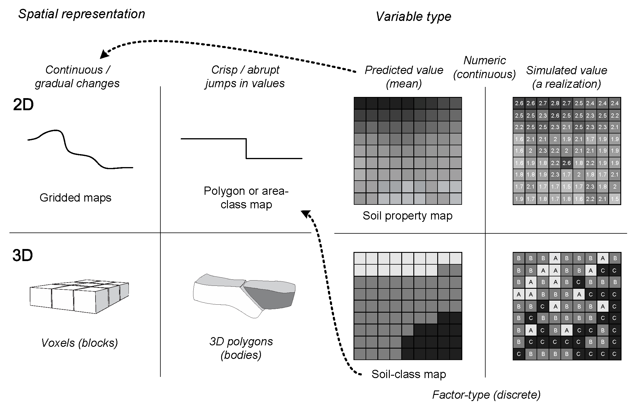
de Gruijter, J. J., D. J. J. Walvoort, and P. F. M. van Gaans. 1997. “Continuous Soil Maps — a Fuzzy Set Approach to Bridge the Gap Between Aggregation Levels of Process and Distribution Models.” Geoderma 77 (2-4):169–95.

McBratney, A. B., M. L. Mendoça Santos, and B. Minasny. 2003. “On digital soil mapping.” Geoderma 117 (1-2):3–52.

Kempen, B., D.J. Brus, G.B.M. Heuvelink, and J.J. Stoorvogel. 2009. “Updating the 1:50,000 Dutch soil map using legacy soil data: A multinomial logistic regression approach.” Geoderma 151 (3-4):311–26. https://doi.org/10.1016/j.geoderma.2009.04.023.

Odgers, Nathan P., Alex B. McBratney, and Budiman Minasny. 2011. “Bottom-up Digital Soil Mapping. II. Soil Series Classes.” Geoderma 163 (1-2):30–37. https://doi.org/10.1016/j.geoderma.2011.03.013.

Wösten, J.H.M., Y.A. Pachepsky, and W.J. Rawls. 2001. “Pedotransfer functions: Bridging the gap between available basic soil data and missing soil hydraulic functions.” Journal of Hydrology 251:123–50.

Wösten, J.H.M., S.J.E. Verzandvoort, J.G.B. Leenaars, T. Hoogland, and J.G. Wesseling. 2013. “Soil Hydraulic Information for River Basin Studies in Semi-Arid Regions.” Geoderma 195. Elsevier:79–86. https://doi.org/10.1016/j.geoderma.2012.11.021.

Dobos, E., F. Carré, T. Hengl, H. I. Reuter, and G. Tóth. 2006. Digital Soil Mapping: As a Support to Production of Functional Maps. Luxemburg: Office for Official Publications of the European Communities.

Burrough, P. A., and R. A. McDonnell. 1998. Principles of Geographical Information Systems. 2nd ed. Oxford: Oxford University Press.

Burrough, P. A., P.H. T. Beckett, and M.G. Jarvis. 1971. “The Relation Between Cost and Utility in Soil Survey (I–Iii).” Journal of Soil Science 22 (3). Blackwell Publishing Ltd:359–94. https://doi.org/10.1111/j.1365-2389.1971.tb01624.x.

Avery, B. 1987. Soil Survey Methods: A Review. Technical Monograph No. 18. Silsoe: Soil Survey & Land Resource Centre.

Legros, J.-P. 2006. Mapping of the Soil. 1st ed. Enfield, New Hampshire: Science Publishers.

Miller, F. P., D. E. McCormack, and J. R. Talbot. 1979. “The Mechanics of Track Support, Piles and Geotechnical Data.” In, 57–65. Symposium, Trans. Res. Record 733. Washington D.C.: Board. Natl. Acad. Sci.

Hudson, B. D. 2004. “The soil survey as a paradigm-based science.” Soil Science Society of America Journal 56:836–41.

Jenny, H. 1994. Factors of Soil Formation: A System of Quantitative Pedology. Dover Books on Earth Sciences. Dover Publications.

McBratney, A.B, M.L Mendonça Santos, and B Minasny. 2003. “On Digital Soil Mapping.” Geoderma 117 (1):3–52. https://doi.org/10.1016/S0016-7061(03)00223-4.

Goovaerts, Pierre. 2001. “Geostatistical Modelling of Uncertainty in Soil Science.” Geoderma 103 (1). Elsevier:3–26.

Hengl, Tomislav, Gerard Heuvelink, and David G Rossiter. 2007. “About Regression-Kriging: From Equations to Case Studies.” Computers & Geosciences 33 (10). Elsevier:1301–15.

MacMillan, R. A., W. W. Pettapiece, and J. A. Brierley. 2005. “An Expert System for Allocating Soils to Landforms Through the Application of Soil Survey Tacit Knowledge.” Canadian Journal of Soil Science, 103–12.

Schelling, J. 1970. “Soil Genesis, Soil Classification and Soil Survey.” Geoderma 4 (3):165–93. https://doi.org/10.1016/0016-7061(70)90002-9.

Soil Survey Staff. 1983. Soil Survey Manual. Rev. Vol. Handbook 18. Washington: United States Agriculture, USDA.

Rossiter, D.G. 2003. Methodology for Soil Resource Inventories. 3rd ed. ITC Lecture Notes Sol.27. Enschede, the Netherlands: ITC.

Zhu, A.X., B. Hudson, J. Burt, K. Lubich, and D. Simonson. 2001. “Soil Mapping Using Gis, Expert Knowledge, and Fuzzy Logic.” Soil Science Society of America Journal 65:1463–72.

Marsman, B.A., and J.J. de Gruijter. 1986. Quality of Soil Maps: A Comparison of Soil Survey Methods in a Sandyarea. Vol. 15. Soil Survey Papers. Wageningen: Netherlands Soil Survey Institute.

Finke, P. 2006. “Quality assessment of digital soil maps: producers and users perspectives.” In Digital Soil Mapping: An Introductory Perspective, edited by P. Lagacherie, A. B. McBratney, and M. Voltz, 523–41. Developments in Soil Science. Amsterdam: Elsevier.

MacMillan, R. A., D.E. Moon, R. A. Coupé, and N. Phillips. 2010. “Predictive Ecosystem Mapping (Pem) for 8.2 Million Ha of Forestland,British Columbia, Canada.” In Digital Soil Mapping: Bridging Research, Environmental Application, and Operation, edited by J. L. Boettinger et al., 2:335–54. Progress in Soil Science. Springer. https://doi.org/10.1007/978-90-481-8863-5_27.

Rosenbaum, U., H. R. Bogena, M. Herbst, J. A. Huisman, T. J. Peterson, A. Weuthen, A. W. Western, and H. Vereecken. 2012. “Seasonal and Event Dynamics of Spatial Soil Moisture Patterns at the Small Catchment Scale.” Water Resources Research 48 (10):1–22. https://doi.org/10.1029/2011WR011518.

Gasch, Caley, Tomislav Hengl, Benedikt Gräler, Hanna Meyer, Troy Magney, and David Brown. 2015. “Spatio-temporal interpolation of soil water, temperature, and electrical conductivity in 3D+T: The Cook Agronomy Farm data set.” Spatial Statistics 14 (Part A):70–90. https://doi.org/10.1016/j.spasta.2015.04.001.

Hengl, Gerard B.M. AND Kempen, Tomislav AND Heuvelink. 2015. “Mapping Soil Properties of Africa at 250 m Resolution: Random Forests Significantly Improve Current Predictions.” PLoS ONE 10 (e0125814). Public Library of Science. https://doi.org/10.1371/journal.pone.0125814.

Grunwald, S. 2005a. Environmental Soil-Landscape Modeling: Geographic Information Technologies and Pedometrics. Books in Soils, Plants, and the Environment Series. Taylor & Francis.

Lagacherie, P., A. B. McBratney, and M. Voltz, eds. 2006. Digital Soil Mapping: An Introductory Perspective. Developments in Soil Science. Amsterdam: Elsevier.

Hartemink, Alfred E., Alex McBratney, and Maria de Lourdes Mendonça-Santos, eds. 2008. Digital Soil Mapping with Limited Data. Vol. 1. Progress in Soil Science. Springer.

Boettinger, J. L., D. W. Howell, A. C. Moore, A. E. Hartemink, and S. Kienast-Brown, eds. 2010. Digital Soil Mapping: Bridging Research, Environmental Application, and Operation. Vol. 2. Progress in Soil Science. Springer.

Franklin, J. 1995. “Predictive Vegetation Mapping: Geographic Modelling of Biospatial Patterns in Relation to Environmental Gradients.” Progress in Physical Geography 19 (4):474–99.

Hengl, Tomislav, Markus G. Walsh, Jonathan Sanderman, Ichsani Wheeler, Sandy P. Harrison, and Iain C. Prentice. 2018. “Global Mapping of Potential Natural Vegetation: An Assessment of Machine Learning Algorithms for Estimating Land Potential.” PeerJ 6 (August):e5457. https://doi.org/10.7717/peerj.5457.

Malone, B.P., B. Minasny, and A.B. McBratney. 2016. Using R for Digital Soil Mapping. Progress in Soil Science. Springer International Publishing.

McBratney, A.B., B. Minasny, and U. Stockmann. 2018. Pedometrics. Progress in Soil Science. Springer International Publishing.

Kondolf, G.M., and H. Piégay. 2003. Tools in Fluvial Geomorphology. Wiley.

Pebesma, E.J. 2006. “The Role of External Variables and GIS Databases in Geostatistical Analysis.” Transactions in GIS 10 (4):615–32.

McBratney, A. B., B. Minasny, R. A. MacMillan, and F. Carré. 2011. “Digital Soil Mapping.” In Handbook of Soil Science, edited by H. Li and M.E. Sumner, 37:1–45. CRC Press.

Zhong, B., and Y.J. Xu. 2011. “Scale Effects of Geographical Soil Datasets on Soil Carbon Estimation in Louisiana, Usa: A Comparison of Statsgo and Ssurgo.” Pedosphere 21 (4):491–501. https://doi.org/10.1016/S1002-0160(11)60151-3.

Henderson, B. L., E. N. Bui, C. J. Moran, and D. A. P. Simon. 2004. “Australia-wide predictions of soil properties using decision trees.” Geoderma 124 (3-4):383–98.

Mansuy, Nicolas, Evelyne Thiffault, David Pare, Pierre Bernier, Luc Guindon, Philippe Villemaire, Vincent Poirier, and Andre Beaudoin. 2014. “Digital Mapping of Soil Properties in Canadian Managed Forests at 250 M of Resolution Using the K-Nearest Neighbor Method.” Geoderma 235-236 (0):59–73. https://doi.org/10.1016/j.geoderma.2014.06.032.

Rowe, J. Stan, and John W. Sheard. 1981. “Ecological Land Classification: A Survey Approach.” Environmental Management 5 (5). Springer:451–64.

Gibbons, Frank R., Ronald Geoffrey Downes, and others. 1964. A study of the land in south-western Victoria. Soil Conservation Authority Melbourne.

Rowan, James Niall. 1990. Land Systems of Victoria. Land Protection Division.

Ramcharan, Amanda, Tomislav Hengl, Travis Nauman, Colby Brungard, Sharon Waltman, Skye Wills, and James Thompson. 2018a. “Soil Property and Class Maps of the Conterminous United States at 100-Meter Spatial Resolution.” Soil Science Society of America Journal 82. The Soil Science Society of America, Inc.:186–201.

Schoeneberger, P.J., D.A. Wysocki, E.C. Benham, and W.D. Broderson. 1998. Field Book for Describing and Sampling Soils. Lincoln, Nebraska: Natural Resources Conservation Service, USDA, National Soil Survey Centre.

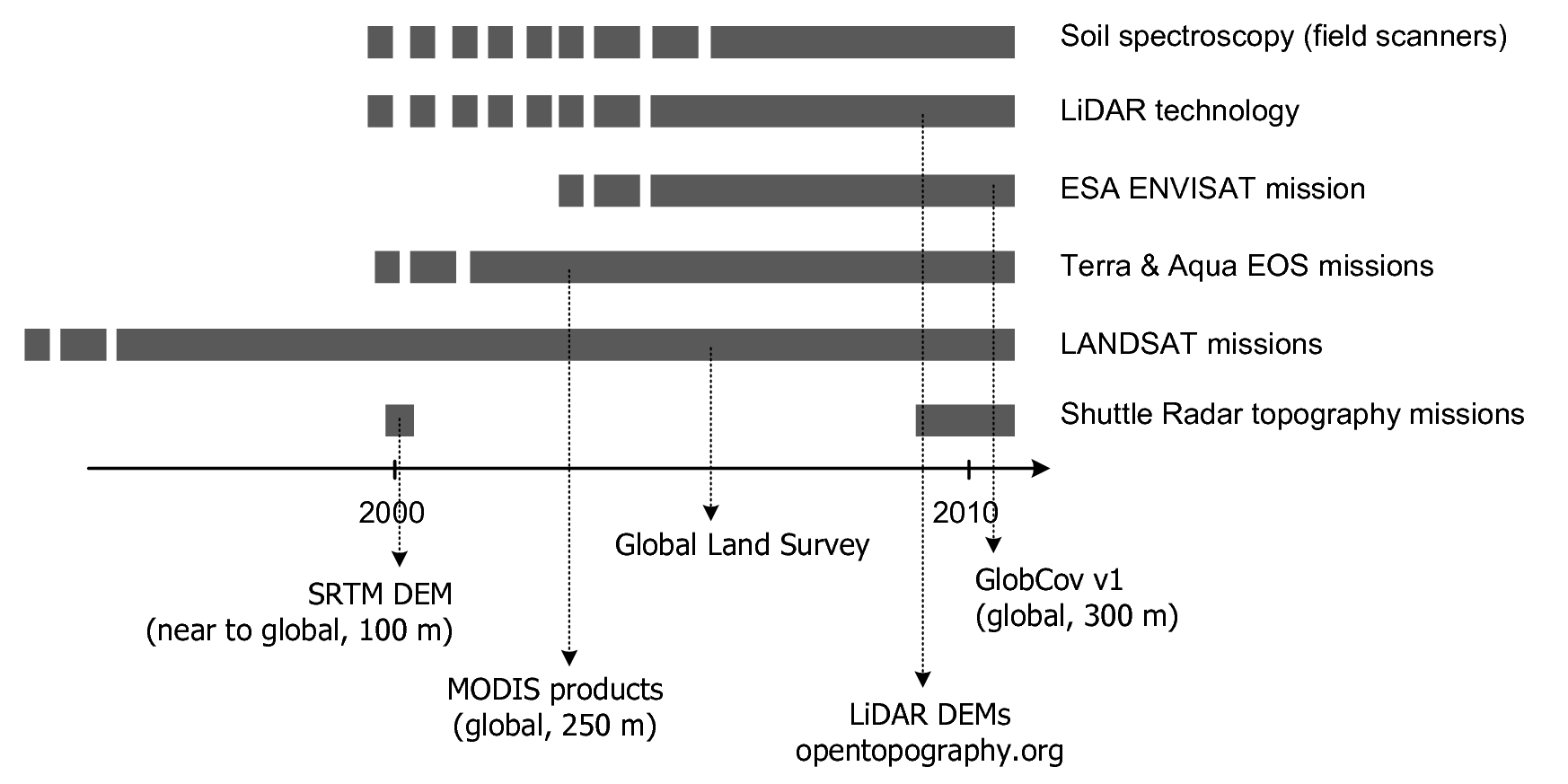
Gehl, RonaldJ., and CharlesW. Rice. 2007. “Emerging Technologies for in Situ Measurement of Soil Carbon.” Climatic Change 80 (1-2). Kluwer Academic Publishers:43–54. https://doi.org/10.1007/s10584-006-9150-2.

Shepherd, K.D., and M.G. Walsh. 2007. “Infrared Spectroscopy — Enabling an Evidence Based Diagnostic Survellance Approach to Agricultural and Environmental Management in Developing Countries.” Journal of Near Infrared Spectroscopy 15:1–19.

Sanchez et al. 2009. “Digital Soil Map of the World.” Science 325:680–81.

Hartemink, A. E., J. Hempel, P. Lagacherie, A. B. McBratney, N. McKenzie, R. A. MacMillan, B. Minasny, et al. 2010. “GlobalSoilMap.net — A New Digital Soil Map of the World.” In Digital Soil Mapping: Bridging Research, Environmental Application, and Operation, edited by J. L. Boettinger, D. W. Howell, A. C. Moore, A. E. Hartemink, and S. Kienast-Brown, 2:423–27. Progress in Soil Science. Springer.

Leenaars, Johan G.B. 2014. Africa Soil Profiles Database, Version 1.2. A Compilation of Geo-Referenced and Standardized Legacy Soil Profile Data for Sub Saharan Africa (with Dataset). Wageningen, the Netherlands: Africa Soil Information Service (AfSIS) project; ISRIC — World Soil Information.

Omuto, C., F. Nachtergaele, and R. Vargas Rojas. 2012. State of the Art Report on Global and Regional Soil Information: Where are we? Where to go? Global Soil Partnership Technical Report. Rome: FAO.

White, R.E. 2009. Principles and Practice of Soil Science: The Soil as a Natural Resource. Wiley.

Simonson, Roy W. 1968. “Concept of Soil.” In Prepared Under the Auspices of the American Society of Agronomy, edited by A.G. Norman, 20:1–47. Advances in Agronomy. Academic Press. https://doi.org/10.1016/S0065-2113(08)60853-6.

Hartemink, Alfred. 2008. “Soil Map Density and a Nation’s Wealth and Income.” In Digital Soil Mapping with Limited Data, edited by Alfred Hartemink, Alex McBratney, and Mariade Lourdes Mendonça-Santos, 53–66. Springer Netherlands. https://doi.org/10.1007/978-1-4020-8592-5_1.

Heuvelink, G.B.M., and R. Webster. 2001. “Modelling soil variation: past, present, and future.” Geoderma 100 (3-4).

Rossiter, D.G. 2003. Methodology for Soil Resource Inventories. 3rd ed. ITC Lecture Notes Sol.27. Enschede, the Netherlands: ITC.

2004. “Digital Soil Resource Inventories: Status and Prospects.” Soil Use and Management 20 (3). Blackwell Publishing Ltd:296–301. https://doi.org/10.1111/j.1475-2743.2004.tb00372.x.

Lathrop Jr., Richard G., John D. Aber, and John A. Bognar. 1995. “Spatial Variability of Digital Soil Maps and Its Impact on Regional Ecosystem Modeling.” Ecological Modelling 82 (1):1–10. https://doi.org/10.1016/0304-3800(94)00068-S.

Bui, E. 2003. “A Strategy to Fill Gaps in Soil Survey over Large Spatial Extents: An Example from the Murray-Darling Basin of Australia.” Geoderma 111:21–44. https://doi.org/10.1016/S0016-7061(02)00238-0.

Grinand, C., D. Arrouays, B. Laroche, and M. Martin. 2008. “Extrapolating regional soil landscapes from an existing soil map: Sampling intensity, validation procedures, and integration of spatialcontext.” Geoderma 143:180–90. https://doi.org/10.1016/j.geoderma.2007.11.004.

Hengl, Tomislav, and Stjepan Husnjak. 2006. “Evaluating Adequacy and Usability of Soil Maps in Croatia.” Soil Science Society of America Journal 70 (3):920–29. https://doi.org/10.2136/sssaj2004.0141.

D’Avello, T.P., and R.L. McLeese. 1998. “Why Are Those Lines Placed Where They Are? An Investigation of Soil Map Recompilation Methods.” Soil Survey Horiz. 39:119–26.

Bui, E. 2004. “Soil Survey as a Knowledge System.” Geoderma 120:17–26. https://doi.org/10.1016/j.geoderma.2003.07.006.

McBratney, Alex, Nathan Odgers, and Budiman Minasny. 2006. “Random Catena Sampling for Establishing Soil-Landscape Rules forDigital Soil Mapping.” In 18th World Congress of Soil Science, 4. Philadelphia, Pennsylvania: IUSS.

Walter, C., P. Lagacherie, and S. Follain. 2006. “Integrating Pedological Knowledge into Digital Soil Mapping.” In Digital Soil Mapping — an Introductory Perspective, edited by P. Lagacherie, A. B. McBratney, and M. Voltz, 31:281–300, 615. Developments in Soil Science. Elsevier. https://doi.org/10.1016/S0166-2481(06)31022-7.

Lagacherie, P. 1995. “A Soil Survey Procedure Using the Knowledge of Soil Pattern Established on a Previously Mapped Reference Area.” Geoderma 65:283–301. https://doi.org/10.1016/0016-7061(94)00040-H.

Lagacherie, P. 2001. “Mapping of Reference Area Representativity Using a Mathematical Soilscape Distance.” Geoderma 101:105–18. https://doi.org/10.1016/S0016-7061(00)00101-4.

Christakos, G., P. Bogaert, and M.L. Serre. 2001. Temporal GIS: advanced functions for field-based applications. v. 1. Springer.

Zhou, Bin, Xin-gang Zhang, and Ren-chao Wang. 2004. “Automated Soil Resources Mapping Based on Decision Tree and Bayesian Predictive Modeling.” Journal of Zhejiang University Science 5:782–95. https://doi.org/10.1631/jzus.2004.0782.

Hengl, T., J. Mendes de Jesus, G. B. M. Heuvelink, M. Ruiperez Gonzalez, M. Kilibarda, A. Blagotic, W. Shangguan, et al. 2017. “SoilGrids250m: Global Gridded Soil Information Based on Machine Learning.” PLoS One 12 (2):e0169748.

Lei, Simon A. 1998. “Soil Properties of the Kelso Sand Dunes in the Mojave Desert.” The Southwestern Naturalist 43 (1). Southwestern Association of Naturalists:47–52.

Raup, Bruce, Adina Racoviteanu, Siri Jodha Singh Khalsa, Christopher Helm, Richard Armstrong, and Yves Arnaud. 2007. “The GLIMS geospatial glacier database: a new tool for studying glacier change.” Global and Planetary Change 56 (1). Elsevier:101–10.

Beaudette, D., and A.T. O’Geen. 2009. “Soil-web: An online soil survey for California, Arizona, and Nevada.” Computers & Geosciences 35:2119–28.

Campbell, Andrew. 2008. Managing Australia’s Soils: A policy discussion paper. Canberra: CSIRO.

Goodchild, M.F. 2008. “Spatial Accuracy 2.0.” In Proceedings of the 8th International Symposium on Spatial Accuracy Assessment in Natural Resources and Environmental Sciences, edited by Wan, Y. et al., 1–7. World Academic Union (Press).

O’Geen, Anthony, Mike Walkinshaw, and Dylan Beaudette. 2017. “SoilWeb: A Multifaceted Interface to Soil Survey Information.” Soil Science Society of America Journal 81 (4). The Soil Science Society of America, Inc.:853–62.

Harpstead, M.I., T.J. Sauer, and W.F. Bennett. 2001. Soil Science Simplified. Wiley.

Walker, W.E., P. Harremoës, J. Rotmans, J.P. van der Sluijs, M.B.A. van Asselt, P. Janssen, and M.P.K von Krauss. 2003. “Defining Uncertainty: A Conceptual Basis for Uncertainty Management in Model-Based Decision Support.” Integrated Assessment 4 (1):5–17.

Refsgaard, Jens Christian, Jeroen P. van der Sluijs, Anker Lajer Højberg, and Peter A. Vanrolleghem. 2007. “Uncertainty in the environmental modelling process — A framework and guidance.” Environ. Model. Softw. 22 (11):1543–56. https://doi.org/10.1016/j.envsoft.2007.02.004.

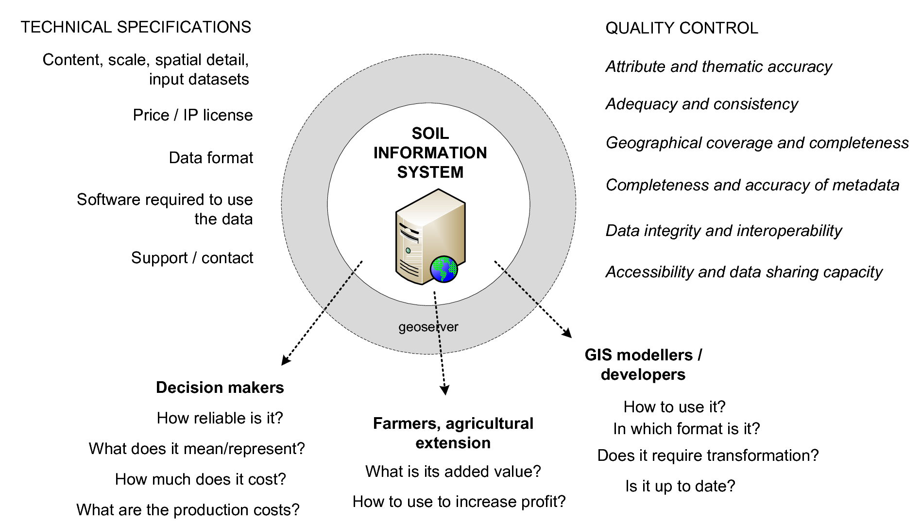
Heuvelink, G.B.M., and J. Brown. 2006. “Towards a Soil Information System for Uncertain Soil Data.” In Digital Soil Mapping: An Introductory Perspective, edited by P. Lagacherie, A. B. McBratney, and M. Voltz, 112–18. Developments in Soil Science. Amsterdam: Elsevier.

Panagos, Panos, Roland Hiederer, Marc Van Liedekerke, and Francesca Bampa. 2013. “Estimating soil organic carbon in Europe based on data collected through an European network.” Ecological Indicators 24 (0):439–50. https://doi.org/10.1016/j.ecolind.2012.07.020.

Kuhn, Max, and Kjell Johnson. 2013. Applied Predictive Modeling. Vol. 810. Springer.

Brus, D.J., B. Kempen, and G.B.M. Heuvelink. 2011. “Sampling for Validation of Digital Soil Maps.” European Journal of Soil Science 62 (3). Blackwell Publishing Ltd:394–407. https://doi.org/10.1111/j.1365-2389.2011.01364.x.

Heuvelink, Gerard BM. 2014. “Uncertainty Quantification of Globalsoilmap Products.” In GlobalSoilMap: Basis of the Global Spatial Soil Information System, edited by D. Arrouays, N. McKenzie, J. Hempel, A.R. de Forges, and A.B. McBratney, 327–32. Taylor & Francis.

Pleijsier, L.K. 1984. Laboratory Methods and Data Quality. Program for Soil Characterization: A Report on the Pilot Round. Part Ii. Exchangeable Bases, Base Saturation and pH. Wageningen: International Soil Reference; Information Centre.

1986. The Laboratory Methods and Data Exchange Programme. Interim Report on the Exchange Round 85-2. Wageningen: International Soil Reference; Information Centre.

van Reeuwijk, L.R. 1982. “Laboratory Methods and Data Quality. Program for Soil Characterization: A Report on the Pilot Round. Part I. CEC and Texture.” In Proceedings of 5th International Classification Workshop. Khartoum, Sudan: ISRIC.

Pleijsier, L.K. 1984. Laboratory Methods and Data Quality. Program for Soil Characterization: A Report on the Pilot Round. Part Ii. Exchangeable Bases, Base Saturation and pH. Wageningen: International Soil Reference; Information Centre.

Lagacherie, P. 1992. “Formalisation Des Lois de Distribution Des Sols Pour Automatiser La Cartographie Pédologique à Partir d’un Secteur Pris Comme Référence. Cas de La Petite Région ‘Moyenne Vallée de L’Hérault’.” PhD thesis, Montpellier: Université des Sciences et Techniques du Languedoc.

Oreskes, Naomi, Kristin Shrader-Frechette, and Kenneth Belitz. 1994. “Verification, Validation, and Confirmation of Numerical Models in the Earth Sciences.” Science 263 (5147):641–46. https://doi.org/10.1126/science.263.5147.641.

Kempen, B., D.J. Brus, and J.J. Stoorvogel. 2011. “Three-Dimensional Mapping of Soil Organic Matter Content Using Soil Type-Specific Depth Functions.” Geoderma 162 (1-2):107–23. https://doi.org/10.1016/j.geoderma.2011.01.010.